41.1 Introduction
In Grade 11 you were introduced to linear programming and solved problems by
looking at points
on the edges of the feasible region. In Grade 12 you will look at how to solve
linear programming
problems in a more general manner.
41.2 Terminology
Here is a recap of some of the important concepts in linear programming.
41.2.1 Feasible Region and Points
Constraints mean that we cannot just take any x and y when looking for the x and
y that
optimise our objective function. If we think of the variables x and y as a point
(x,y) in the xy-
plane then we call the set of all points in the xy-plane that satisfy our
constraints the feasible
region. Any point in the feasible region is called a feasible point.
For example, the constraints
x ≥ 0
y ≥ 0
mean that every (x,y) we can consider must lie in the first quadrant of the
xy plane. The
constraint
x ≥ y
means that every (x,y) must lie on or below the line y = x and the constraint
x ≤ 20
means that x must lie on or to the left of the line x = 20.
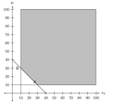
We can use these constraints to draw the feasible region as shown by the
shaded region in
Figure 41.1.
Important: The constraints are used to create bounds of the solution.
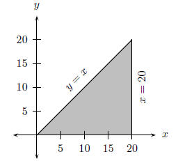
Figure 41.1: The feasible region corresponding to the constraints x ≥ 0, y ≥
0, x ≥ y and
x ≤ 20.
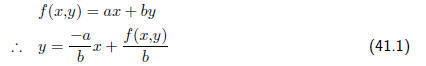
Important:
| ax + by = c |
If b ≠ 0, feasible points must lie on the
line

If b = 0, feasible points must lie on the line
x = c/a |
| ax + by ≤ c |
If b ≠ 0, feasible points must lie on or
below the
line
.
If b = 0, feasible points must lie on or to the left
of the line x = c/a. |
When a constraint is linear, it means that it requires that any feasible
point (x,y) lies on one
side of or on a line. Interpreting constraints as graphs in the xy plane is very
important since it
allows us to construct the feasible region such as in Figure 41.1.
41.3 Linear Programming and the Feasible Region
If the objective function and all of the constraints are linear then we call
the problem of optimising
the objective function subject to these constraints a linear program. All
optimisation problems
we will look at will be linear programs.
The major consequence of the constraints being linear is that the feasible
region is always a
polygon. This is evident since the constraints that define the feasible region
all contribute a line
segment to its boundary (see Figure 41.1). It is also always true that the
feasible region is a
convex polygon.
The objective function being linear means that the feasible point(s) that
gives the solution of a
linear program always lies on one of the vertices of the feasible region. This
is very important
since, as we will soon see, it gives us a way of solving linear programs.
We will now see why the solutions of a linear program always lie on the
vertices of the feasible
region. Firstly, note that if we think of f(x,y) as lying on the z axis, then
the function f(x,y) =
ax + by (where a and b are real numbers) is the definition of a plane. If we
solve for y in the
equation defining the objective function then
What this means is that if we find all the points where f(x,y) = c for any
real number c (i.e.
f(x,y) is constant with a value of c), then we have the equation of a line. This
line we call a
level line of the objective function.
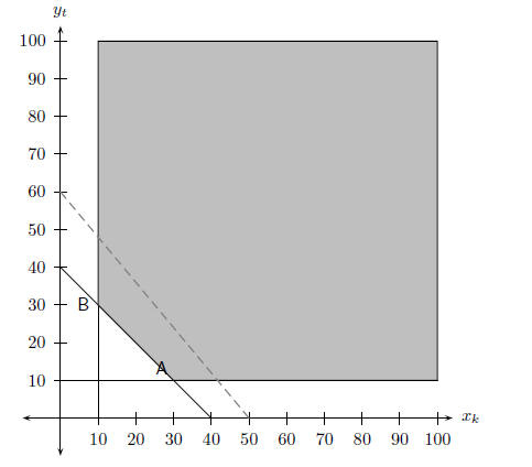
Consider again the feasible region described in Figure 41.1. Lets say that we
have the objective
function f(x,y) = x− 2y with this feasible region. If we consider Equation ??
corresponding to
f(x,y) = −20
then we get the level line

which has been drawn in Figure 41.2. Level lines corresponding to
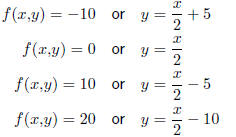
have also been drawn in. It is very important to realise that these are not
the only level lines; in
fact, there are infinitely many of them and they are all parallel to each other.
Remember that if
we look at any one level line f(x,y) has the same value for every point (x,y)
that lies on that
line. Also, f(x,y) will always have different values on different level lines.
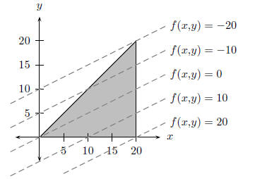
Figure 41.2: The feasible region corresponding to the constraints x ≥ 0, y ≥
0, x ≥ y and
x ≤ 20 with objective function f(x,y) = x − 2y. The dashed lines represent
various level lines
of f(x,y).
If a ruler is placed on the level line corresponding to f(x,y) = −20 in
Figure 41.2 and moved
down the page parallel to this line then it is clear that the ruler will be
moving over level lines
which correspond to larger values of f(x,y). So if we wanted to maximise f(x,y)
then we simply
move the ruler down the page until we reach the “ lowest ” point in the feasible
region. This point
will then be the feasible point that maximises f(x,y). Similarly, if we wanted
to minimise f(x,y)
then the “highest” feasible point will give the minimum value of f(x,y).
Since our feasible region is a polygon, these points will always lie on
vertices in the feasible
region. The fact that the value of our objective function along the line of the
ruler increases
as we move it down and decreases as we move it up depends on this particular
example. Some
other examples might have that the function increases as we move the ruler up
and decreases
as we move it down.
It is a general property , though, of linear objective functions that they
will consistently increase
or decrease as we move the ruler up or down. Knowing which direction to move the
ruler in
order to maximise /minimise f(x,y) = ax + by is as simple as looking at the sign
of b (i.e. “is
b negative , positive or zero ?”). If b is positive, then f(x,y) increases as we
move the ruler up
and f(x,y) decreases as we move the ruler down. The opposite happens for the
case when b is
negative: f(x,y) decreases as we move the ruler up and f(x,y) increases as we
move the ruler
down. If b = 0 then we need to look at the sign of a.
If a is positive then f(x,y) increases as we move the ruler to the right and
decreases if we move
the ruler to the left. Once again, the opposite happens for a negative. If we
look again at the
objective function mentioned earlier,
f(x,y) = x − 2y
with a = 1 and b = −2, then we should find that f(x,y) increases as we move
the ruler down
the page since b = −2 < 0. This is exactly what we found happening in Figure
41.2.
The main points about linear programming we have encountered so far are
• The feasible region is always a polygon.
• Solutions occur at vertices of the feasible region.
• Moving a ruler parallel to the level lines of the objective function up/down
to the top/bottom
of the feasible region shows us which of the vertices is the solution.
• The direction in which to move the ruler is determined by the sign of b and
also possibly
by the sign of a.
These points are sufficient to determine a method for solving any linear
program.
Method: Linear Programming
If we wish to maximise the objective function f(x,y) then:
1. Find the gradient of the level lines of f(x,y) (this is always going to be
−a/b as we saw in
Equation ??)
2. Place your ruler on the xy plane, making a line with gradient −a/b (i.e. b
units on the
x-axis and −a units on the y-axis)
3. The solution of the linear program is given by appropriately moving the
ruler. Firstly we
need to check whether b is negative, positive or zero .
A If b > 0, move the ruler up the page, keeping the ruler parallel to the
level lines all
the time, until it touches the “highest” point in the feasible region. This
point is
then the solution.
B If b < 0, move the ruler in the opposite direction to get the solution at the
“lowest”
point in the feasible region.
C If b = 0, check the sign of a
i. If a < 0 move the ruler to the “leftmost” feasible point. This point
is then the
solution.
ii. If a > 0 move the ruler to the “rightmost” feasible point. This point
is then the
solution.
Worked Example 188: Prizes!
Question: As part of their opening specials, a furniture store has
promised to give
away at least 40 prizes with a total value of at least R2 000. The prizes are
kettles
and toasters.
1. If the company decides that there will be at least 10 of each prize, write
down
two more inequalities from these constraints.
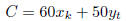
2. If the cost of manufacturing a kettle is R60 and a toaster is R50, write down
an
objective function C which can be used to determine the cost to the company
of both kettles and toasters.
3. Sketch the graph of the feasibility region that can be used to determine all
the
possible combinations of kettles and toasters that honour the promises of the
company.
4. How many of each prize will represent the cheapest option for the company?
5. How much will this combination of kettles and toasters cost?
Answer
Step 1 : Identify the decision variables
Let the number of kettles be xk and the number of toasters be yt and write down
two constraints apart from xk ≥ 0 and yt ≥ 0 that must be adhered to.
Step 2 : Write constraint equations
Since there will be at least 10 of each prize we can write:

and

Also the store has promised to give away at least 40
prizes in total. Therefore:

Step 3 : Write the objective function
The cost of manufacturing a kettle is R60 and a toaster is R50. Therefore the
cost
the total cost C is:
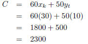
Step 4 : Sketch the graph of the feasible region
Step 5 : Determine vertices of feasible region
From the graph, the coordinates of vertex A is (3,1) and the coordinates of
vertex
B are (1,3).
Step 6 : Draw in the search line
The seach line is the gradient of the objective function. That is, if the
equation
C = 60x + 50y is now written in the standard form y = ..., then the gradient is:

which is shown with the broken line on the graph.
Step 7 : Calculate cost at each vertex
At vertex A , the cost is:
At vertex B, the cost is:
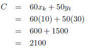
Step 8 : Write the final answer
The cheapest combination of prizes is 10 kettles and 30 toasters, costing the
company
R2 100.
Worked Example 189: Search Line Method
Question: As a production planner at a factory
manufacturing lawn cutters your job
will be to advise the management on how many of each model should be produced
per
week in order to maximise the profit on the local production. The factory is
producing
two types of lawn cutters: Quadrant and Pentagon. Two of the production
processes
that the lawn cutters must go through are: bodywork and engine work.
• The factory cannot operate for less than 360 hours on
engine work for the lawn
cutters.
• The factory has a maximum capacity of 480 hours for bodywork for the lawn
cutters.
• Half an hour of engine work and half an hour of bodywork is required to
produce
one Quadrant.
• One third of an hour of engine work andone fifth of an hour of bodywork is
required to produce one Pentagon.
• The ratio of Pentagon lawn cutters to Quadrant lawn cutters produced per
week must be at least 3:2.
• A minimum of 200 Quadrant lawn cutters must be produced per week.
Let the number of Quadrant lawn cutters manufactured in a
week be x.
Let the number of Pentagon lawn cutters manufactured in a week be y.
Two of the constraints are:
x ≥ 200
3x + 2y ≥ 2 160
1. Write down the remaining constraints in terms of x and
y to represent the
abovementioned information.
2. Use graph paper to represent the constraints graphically.
3. Clearly indicate the feasible region by shading it.
4. If the profit on one Quadrant lawn cutter is R1 200 and the profit on one
Pentagon lawn cutter is R400, write down an equation that will represent the
profit on the lawn cutters.
5. Using a search line and your graph, determine the number of Quadrant and
Pentagon lawn cutters that will yield a maximum profit.
6. Determine the maximum profit per week.
Answer
Step 1 : Remaining constraints:
Step 2 : Graphical representation
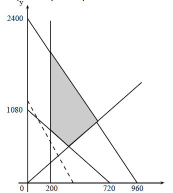
Step 3 : Profit equation
P = 1 200x + 400y
Step 4 : Maximum profit
P = 1 200(600)+ 400(900)
P = R1 080 000
41.4 End of Chapter Exercises
1. Polkadots is a small company that makes two types of
cards, type X and type Y. With the
available labour and material, the company can make not more than 150 cards of
type X
and not more than 120 cards of type Y per week. Altogether they cannot make more
than
200 cards per week.
There is an order for at least 40 type X cards and 10 type
Y cards per week. Polkadots
makes a profit of R5 for each type X card sold and R10 for each type Y card.
Let the number of type X cards be x and the number of type Y cards be y,
manufactured
per week.
A One of the constraint inequalities which represents the
restrictions above is x ≤ 150.
Write the other constraint inequalities.
B Represent the constraints graphically and shade the feasible region.
C Write the equation that represents the profit P (the objective function), in
terms of
x and y.
D On your graph, draw a straight line which will help you to determine how many
of
each type must be made weekly to produce the maximum P
E Calculate the maximum weekly profit.
2. A brickworks produces “face bricks” and “clinkers”.
Both types of bricks are produced and
sold in batches of a thousand. Face bricks are sold at R150 per thousand, and
clinkers at
R100 per thousand, where an income of at least R9,000 per month is required to
cover
costs. The brickworks is able to produce at most 40,000 face bricks and 90,000
clinkers
per month, and has transport facilities to deliver at most 100,000 bricks per
month. The
number of clinkers produced must be at least the same number of face bricks
produced.
Let the number of face bricks in thousands be x, and the number of clinkers in
thousands
be y.
A List all the constraints.
B Graph the feasible region.
C If the sale of face bricks yields a profit of R25 per thousand and clinkers
R45 per
thousand, use your graph to determine the maximum profit.
D If the profit margins on face bricks and clinkers are interchanged, use your
graph to
determine the maximum profit.
3. A small cell phone company makes two types of cell
phones: Easyhear and Longtalk.
Production figures are checked weekly. At most, 42 Easyhear and 60 Longtalk
phones
can be manufactured each week. At least 30 cell phones must be produced each
week to
cover costs. In order not to flood the market, the number of Easyhear phones
cannot be
more than twice the number of Longtalk phones. It takes 2/3 hour to assemble an
Easyhear
phone and 1/2 hour to put together a Longtalk phone. The trade unions only allow
for a
50-hour week.
Let x be the number of Easyhear phones and y be the number of Longtalk phones
man-
ufactured each week.
A Two of the constraints are:
0 ≤ x ≤ 42 and 0 ≤ y ≤ 60
B Draw a graph to represent the feasible region
C If the profit on an Easyhear phone is R225 and the profit on a Longtalk is
R75,
determine the maximum profit per week.
4. Hair for Africa is a firm that specialises in making
two kinds of up-market shampoo,
Glowhair and Longcurls. They must produce at least two cases of Glowhair and one
case
of Longcurls per day to stay in the market. Due to a limited supply of
chemicals, they
cannot produce more than 8 cases of Glowhair and 6 cases of Longcurls per day.
It takes
half-an-hour to produce one case of Glowhair and one hour to produce a case of
Longcurls,
and due to restrictions by the unions, the plant may operate for at most 7 hours
per day.
The workforce at Hair for Africa, which is still in training, can only produce a
maximum
of 10 cases of shampoo per day.
Let x be the number of cases of Glowhair and y the number of cases of Longcurls
produced
per day.
A Write down the inequalities that represent all the
constraints.
B Sketch the feasible region.
C If the profit on a case of Glowhair is R400 and the profit on a case of
Longcurls is
R300, determine the maximum profit that Hair for Africa can make per day.
5. A transport contracter has 6 5-ton trucks and 8 3-ton
trucks. He must deliver at least 120
tons of sand per day to a construction site, but he may not deliver more than
180 tons per
day. The 5-ton trucks can each make three trips per day at a cost of R30 per
trip, and
the 3-ton trucks can each make four trips per day at a cost of R120 per trip.
How must
the contracter utilise his trucks so that he has minimum expense ?