A Functional Link Network With Ordered Basis Functions

Abstract—A procedure is presented for selecting and
ordering the polynomial basis functions in the functional link
net (FLN). This procedure, based upon a modified Gram
Schmidt orthonormalization, eliminates linearly dependent and
less useful basis functions at an early stage, reducing the
possibility of combinatorial explosion. The number of passes
through the training data is minimized through the use of
correlations. A one-pass method is used for validation and
network sizing. Function approximation and learning examples
are presented. Results for the Ordered FLN are compared with
those for the FLN, Group Method of Data Handling, and MultiLayer Perceptron.

I. INTRODUCTION

Multilayer perceptron (MLP) neural nets[1] have proved
useful in many approximation and classification
applications because of their universal approximation
properties [2,3], their relation to optimal approximations [4]
and classifiers [5], and the existence of workable training
algorithms such as backpropagation[1]. They have the
unique property that their basis functions develop during
training rather than being arbitrarily chosen ahead of time.
However, the MLP has long training time, is sensitive to
initial weight choices, and its training error may not
converge to a global minimum. In addition, there is a wide
gap between the MLP’s theoretical capabilities and its actual
performance with currently available training algorithms.
 

In contrast, the functional link network[6] (FLN) has a flat
architecture, with pre-defined basis functions like the
trigonometric functions, algebraic polynomials, Chebyshev
polynomials and Hermite polynomials. The global minimum
of its error function can be found by solving linear equations
[6] or by techniques such as genetic algorithms [7]. As with
other Polynomial Neural Networks (PNN) faster learning
rates are achieved [8] for a given network-size.

However, with an increase in degree of approximation and
inputs there is a combinatorial explosion in the number of
basis functions required during training. This is the biggest
drawback in application of the FLN. Several other PNNs
have been developed to remedy this including group method
of data handling (GMDH) networks [9,10], in which many
trial polynomial basis functions are generated, but only those
which prove useful are kept. Pi-sigma networks [11] do not
have the universal approximation property, but Ridged-Polynomial
network [12] may address that problem .

Orthonormal Least Squares (OLS) has been used by Chen
et al. [13] to efficiently find subsets of center vectors in
radial basis function (RBF) networks. Kamniski and
Strumillo [14] used modified Gram Schmidt
orthonormalization (MGSO) to compute hidden weights in
RBF networks.

In this work, we use MGSO to orthonormalize sets of FLN
basis functions and methodically order them according to
their contribution to the decrease in the mean square error
(MSE). The network thus obtained is called the Ordered
FLN (OFLN). In Section 2 the FLN is briefly reviewed. The
notation and structure of the OFLN is introduced in section
3. Section 4 summarizes the MGSO training procedure for
the OFLN. Numerical results in section 5 compare the FLN,
GMDH, MLP and OFLN.

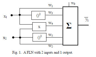
II. FUNCTIONAL LINK NETWORK

FLNs often have a fixed number of polynomial or
trigonometric basis functions. A 2^nd degree FLN with 2
inputs and 1 output is shown in Fig. 1.

This two-input unit can be scaled to a single-layer network
mapping R^N → R^M where N and M respectively denote the
numbers of inputs and outputs. Alternately, several of these
two-input units can be used in a multi-layered network such
as the GMDH. In either case, the resulting network
approximates the Kolmogorov-Gabor or Ivakhnenko
polynomial [10,15]

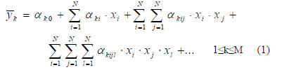
where is the k^th estimated output and α_k’s are the
corresponding coefficients. Let X be a column vector of
basis functions, then the i^th polynomial basis function (PBF)
element X_i is an element of the monomial set
{1,x_i,x_i·x_j,x_i·x_j·x_k,… } for 1≤i≤j≤k…≤N. Now, (1) is rewritten as
 

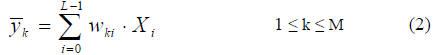
where w_ki connects Xi to the k^th output . For an FLN that
approximates a function with maximum degree monomial D,
the total number of basis functions is given by

Assume that the N-dimensional input vector x has mean
vector m and a vector σ of standard deviations. We
normalize x as

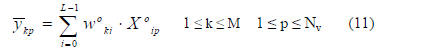
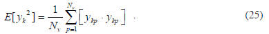
where N_v is the number of training patterns. The bias term x₀
as in (1) is defined to be 1. For the p^th pattern, let y_kp be the
k^th observed or desired output and let X_ip denote the p^th value
of X_i. The error function to be minimized in FLN training is

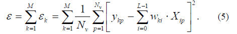
Minimization of (5) can be reduced to solving M sets of L
linear equations in L unknowns .

Clearly the problem of combinatorial explosion with an
increase in D and N is evident from (3), as an example with 5
inputs and 2^nd degree approximation, L is 21 and for 25
inputs and 4^th degree approximation, L is 23751. This makes
it impractical to design and apply high degree FLNs

III. ALGORITHM APPROACH AND NOTATION

In order to prevent combinatorial explosion in the FLN,
we need to limit the value of L. One approach is to limit the
FLN’s degree D. However, this limits its ability to model
complicated functions. A better approach is to use only the
most useful basis functions. If the elements of X are to be in
descending order of usefulness, a method is needed for
generating these elements efficiently, in any possible order.

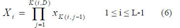
Consider an L by (D+1) position matrix K, whose i^th row
specifies how to generate the PBF X_i. For element K(i,j), the
ranges of i and j are 0 ≤ i ≤ L-1 and 0 ≤ j ≤ D. The i^th PBF,
with K(i,D) denoting its degree, is defined as

The first basis function as in (2) is fixed as X₀ = 1. Thus X
can be generated from K and the normalized input vector x.
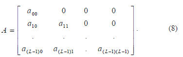
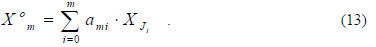
An orthonormalized representation of X is X⁰, which is to be
generated by the transformation

where A is a lower triangular L by L transformation matrix

Given X, as generated by an initial K matrix, let elements of
the array J index basis functions according to their
usefulness. If J₀ = 3 and J₃ = 8, for example, the 1^st and 4^th
most useful basis functions are X₃ and X₈ respectively.

Our general approach for training the OFLN is to
iteratively generate K and J for higher and higher degrees,
D, finding the basis function coefficients each time via
MGSO. In each iteration, redundant and useless basis
functions are eliminated, in order to prevent combinatorial
explosion in the subsequent iterations.

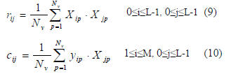
Relevant correlations for MGSO are the auto and crosscorrelation
functions defined as

IV. MODIFIED GRAM SCHMIDT ORTHONORMALIZATION PROCEDURE

The MGSO algorithm orthonormalizes a set of linearly
independent functions or vectors in inner product space . It is
fast and numerically stable and has been used in Least
Square Estimation problems[16], optimal MLP pruning
[17], and in efficient feature selection using piecewise linear
networks (PLN)[18].

In this section we use MGSO to simultaneously
orthonormalize PBFs and solve linear equations for the
OFLN’s weights. Rewriting (2) in terms of p ^th training
pattern of the i^th orthonormal vector ,

where is the transformed weight corresponding to the k^th
output and i^th orthonormal PBF

A. Degree D Up to One

In the first OFLN training iteration, we order the inputs,
discarding those that are linearly dependent or less useful for
estimating outputs. Here, L = N+1 and K and J are
initialized as

Following the basis function definition in (6), (12) indicates
that the maximum degree is D=1, the first basis function is
the constant 1, and the remaining basis functions are inputs.
Our goal is to find the vector J whose elements are indices of
linearly independent inputs, in order of their contribution to
reduce the MSE. The m^th orthonormal basis function

from (7) and (8) is given by

Then for m=0,

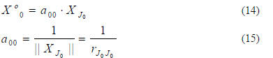
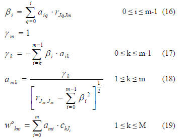
For 1≤m≤L-1, perform the following operations

It can be easily proved that for values of m, is
linearly dependent on previously generated PBFs.

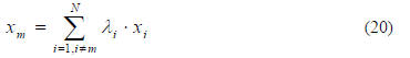
Lemma I: If any input x_m is linearly dependent on other
inputs then higher order basis functions that include x_m can
be expressed using basis functions of the same degree that do
not include x_m.

Proof: For any input x_m that is linearly dependent on other
inputs there exists at least one non-zero λ_i such that

Consider a degree D basis function with dependent input x_m
raised to the d^th power. We have

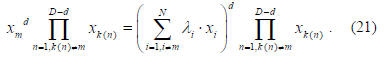
In (21), the right hand side has no x_m and the degree D is
also unchanged. Thus each m^th linearly dependent function
can be eliminated as

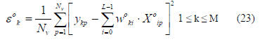
The corresponding MSE for the orthonormal system is given by

The total system error ε can be solved as

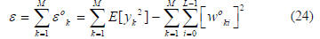
where the expectation operator is given by

Equation (24) measures a basis function’s contribution to
reduce the MSE. Denote the second term in (24) by P_i
associated with i^th orthonormal basis function

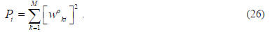
The desired new order of basis functions J that reduces the
MSE is thus obtained by maximizing P_i so that

The orthonormal weights are transformed back to original
weights as

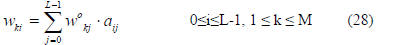
At this point, J gives us the order of the useful basis
functions for a linear network. If only a first order
approximation is required, then a reordered K based on J
and weights as in (28) could be saved and they represent the
OFLN of degree 1.

B. Degree D Greater Than One

As the network grows iteratively for each degree up to the
desired D, the rows of K are reordered based on J that
constitute only essential PBFs. Following lemma 1, rows of
K describing new candidate basis functions are generated by
unique combinations of existing rows of K and appended to
it. Equations (14)-(19), (22)-(24), (26)-(27) are repeated with
the value of L being the row count of K for each degree. As
a control or stopping criterion, we can stop at a given
maximum number of PBF’s L_max. Alternately, we can stop
when the percentage change in error for adding a PBF is less
than a user-chosen value . The MSE is a monotonically
non-increasing function for increase in L as seen from (24).

C. One-Pass Validation

As with other nonlinear networks, there are no practical
optimal approaches for determining network size. The user
can pick a high but practical degree D, and find the number
of basis functions that minimizes validation error.

However, using MGSO, a one-pass measurement of
validation error for network size up to L is possible. The
validation dataset is normalized with known values of m and
σ. X, X^o are generated using (6) and (13) respectively. Then,
for a network of size k with N_vt validation patterns, the total
validation MSE (ε_vk) is given by

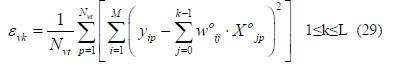
Given the pattern number p, the quantity in the inner
brackets is evaluated for all values of k. Hence ε_vk is
updated for all values of k in a single pass through the data.

The MGSO approach of this section reduces the OFLN’s
computational load in two ways . First, it allows us to greatly
reduce the number of basis functions used in the FLN,
speeding up the design procedure, reducing the
computational load of the network. Second, it leads to a one-pass
validation of OFLNs with many different values of L.

V. COMPARISON AND SIMULATION RESULTS

A. Function approximation

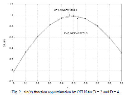
Two examples are given to show the function
approximation capabilities of the OFLN. In the first
example, 10 data values in the interval [0:1] are used for
learning the sine function (Fig. 2) [11]. The OFLN exhibits
small error, as expected.

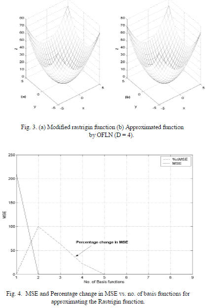
In the second example, a modified rastrigin function
(given by is
approximated by the OFLN (Fig. 3). Fig. 4 shows an
important advantage of the OFLN over FLN, sigma-pi and
GMDH, i.e. as percentage change in MSE is zero then
minimal number of 4 basis functions of up to degree 4 are
sufficient for approximation with MSE = 0.08. Also, from
(3), for N=2, D=4, L would be 15 but 6 of them are linearly
dependent and eliminated during training. Hence, unlike
GMDH and sigma-pi networks there are no repeated and
redundant terms for higher degree representation. Results
show that this property scales extremely well for systems
with large numbers of inputs and outputs.

B. Supervised learning examples

Here, some examples for supervised learning are
demonstrated for the OFLN. For comparison, a GMDH
network [19,20] was designed using the Forward
Prediction Error (FPE) criterion. In examples 1 and 2,
an MLP was trained with back-propagation and the
Levenberg-Marquardt algorithm. In examples 3 and 4
the MLP is trained using Output-Weight-Optimization
Hidden-Weight-Optimization (OWO-HWO)[21].

Errors were averaged for 3 sets of random data with
ratio of 7:3 for training and validation.

The 1^st example is a benchmark function
approximation problem “California Housing” from
Statlib[22]. It has 20,640 observations for predicting the
price of houses in California, with 8 continuous inputs
(median income, housing median age, total rooms, total
bedrooms, population, households, latitude, and
longitude) and one continuous output (median house
value).

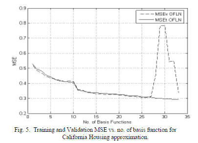
The output was normalized by subtracting the mean and
dividing by the standard deviation. The MSE obtained was
0.30, 0.38 and 0.35 for the OFLN, GMDH and MLP
respectively. OFLN used 27 basis functions with D=4. The
4^th degree GMDH had 27 PBFs. An 8-18-1 MLP used a
validation set for early stopping and converged at 31 epochs.
Fig. 5 shows the training and validation MSEs, MSEt and
MSEv vs. the number of basis function for OFLN with D=4.
As the validation error increases for more than 27 basis
functions, it is selected as a stopping criterion [10].

The 2^nd example comprises an empirical MIMO
geophysical system for surface analysis from polarimetric
radar measurements[23]. There are 20 inputs corresponding
to VV and HH polarization at L 30, 40 deg, C 10, 30, 40, 50,
60 deg, and X 30, 40, 50 deg and 3 outputs corresponding to
rms surface height, surface correlation length, and
volumetric soil moisture content in g/ cubic cm . Fig. 6 shows
the training and validation MSE vs. no. of basis function
graph for ordered PBF’s 1 to 60 for D=4. Results show good
generalization capabilities for the OFLN

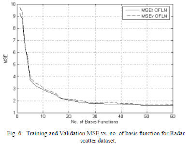
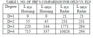
Table 1 compares L values used for the FLN and OFLN in
the California housing and radar applications. Although
L_OFLN for California housing example for D=4 is 377 for
effective generalization only 27 basis functions are
sufficient, as seen in Fig. 5. Table 2 gives the corresponding
training and validation MSE at each degree for the two
applications.

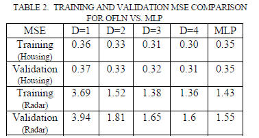
Because of the equation (24), the OFLN’s training MSE is a
monotonically non-increasing function of D and L. Also for
D^th degree learning, the training data need be read only
(D+1) times. These attributes make OFLN training more
computationally efficient than that of the GMDH.

The 3^rd example involves the demodulation of a noisy
Frequency Modulation (FM) samples to recover the bandlimited
signal. If x[n] is the modulating signal, z[n] is the
output of FM modulator with additive noise e[n], then for
modulation index k_f, carrier amplitude A_c, carrier frequency
f_c, modulating signal frequency f_m

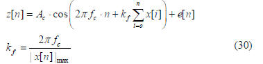
1024 patterns are generated with z[i], 0≤i≤4 as inputs and
desired x[n] as output with values of A_c, f_c, f_m as 0.5, 0.1 and
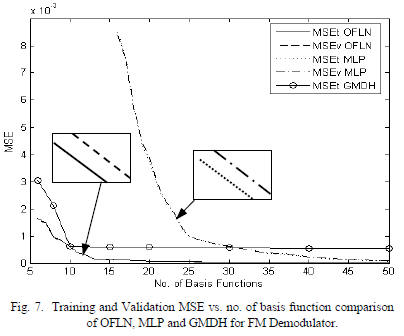
0.1 respectively. Comparison of OFLN, MLP and GMDH
based on training MSE (MSEt) and validation MSE (MSEv)
vs. the number of basis functions is shown in Fig. 7. OFLN
gives a lower MSE for training and validation compared to
MLP and GMDH. The number of basis functions for MLP
under consideration is given by (Number of hidden units + N
+ 1). The GMDH network uses 5^th degree approximation for
50 iterations. Performance results for OFLN are
comparatively better. Also, a system modeler can select a
smaller size OFLN network with a trade-off in MSE, e.g.
OFLN of size 40 compared to OFLN of size 60 has 2%
additional training MSE at cost of 20 more PBF’s.

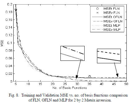
Finally, results for non-linear 2 by 2 matrix inversion
problem are shown in Fig. 8. The training file has 2000
patterns, each with N=M=4. The inputs are uniformly
distributed between 0 and 1, and represent a matrix. The four
desired outputs are elements of the corresponding inverse
matrix. The determinants of the input matrices are
constrained to be between .3 and 2. FLN, OFLN and MLP
networks are compared in Fig. 8. Note that the FLN points
are widely separated, giving the user few options as to
network size.

We see that all three networks perform similarly when the
number of basis functions is 23 or less. However, for this
dataset, the MLP has an advantage for 24 or more basis
functions.

VI. CONCLUSIONS

The OFLN gives a concise, methodically ordered and
computationally efficient representation for supervised, nonparametric
MIMO systems that is a better than that of some
other PNN networks. It reduces the number of passes
through the dataset. It can certainly be applied to many
nonlinear function approximation, structure identification
and optimization problems. The OFLN can be extended to
classification problems as well. Future work will include the
development of computationally more efficient methods for
the generation and index storage of higher order PBFs so as
to enhance the scalability of the network.