5 Data AnalysisWith MATLAB
MATLAB basics will be learned, based on your assigned reading
and class practice. §5.1 and §5.2 are included as immediate reminders. The
discussion of data analysis begins in §5.3.
5.1 Creating & Saving a New M-File on a Memory Stick
MATLAB computations can be executed directly from the MATLAB
command window, or by use of program files. MATLAB programs are saved as
M-files in an accessible directory, as explained below. Since lab computers
will be used by others we shall never save programs on the hard disk.
Here and throughout, programs will be saved as M-files on a memory stick and run
from the appropriate directory.
In what follows we refer to the directory of the memory
stick as “E”. Make sure to check which directory is actually occupied by
the memory stick and substitute the correct reference for “E”.
Files saved on the hard disk might be erased
and lost without prior notice!
• Insert a memory clip
• In the MATLAB command window, change directory to the floppy
drive
>> cd E:\
• Verify the current directory
>>pwd
>> E:\
• Under “File”, select “New M-file”
• Save the new M-file under a name of your choice, with the
suffix “.m” (for example SOS -Lab1.m is a good name for a program used to
measure the speed of sound in Lab 1). The following rules apply to names used
for both
MATLAB variables and M -files:
– the name must begin with a letter
– the name may contain letters, numbers and the underscore
sign
– the name may not contain other characters, or a space
– the name may not be equal to the name of a recognized
MATLAB function (such as sin, cos, log, etc.).
When in doubt, do not use a suspected name
for your variables and programs!
To run an M-file as a
script program, type its name in the
MATLAB workspace
and hit return. Alternatively, select the
run icon in the
editor window.
5.2 Defining MATLAB Variables
This part is covered in the required Lab 1 book reading
and will be practiced in class. The following is are few highlights:
• Variables are used to store data values. The name of the
variable is a reference to a point in the memory.
• MATLAB will not recognize a variable before it is expressly
defined.
To see that type boom in the command window. Assuming a variable
bum was not previously defined , the response will be
>>boom
>>
??? Undefined
function or variable ’boom’.
• The equal sign “=” is used in MATLAB, as in most programming
languages, for the assignment operation, acting from left to right. Thus
>>moom=5
assigns the value 5 to the variable moom. If moom did not
previously exist, it also creates this variable in the memory. Contrary to the
usual usage of “=” in mathematics , the legal operation
>>moom=moom+1
assigns to the existing variable moom a new value, comprising
its old value plus one.
• By default, each value assignment command is followed by a
display of the assigned value in the MATLAB command window. This is mostly
undesirable, and in case of large array, will dramatically slow down you
programs! To prevent this and as a matter of standard practice, end each
assignment command with a semicolon “;”
• Variables may be
scalars (the default), taking a single number (or
character) as a value. They may also be one, two or three dimensional
arrays of values.
Details are provided in the book (pp. 40-48).
5.3 Experimental Data Recording and Plotting
The following commands should be included in an M-file used to
record and plot the data from the speed of sound experiment. Your Lab report
should include the M-file and a printout of the MATLAB command window were the
M-file is executed5
• define three row vectors of size 1 × 10 (remember to type a
semicolon “;” at the end of each vector definition!):
– A vector tdistance whose entries are the 10 distances
between the two transducers in your experiments
– A vector ttime whose entries are the corresponding
measured travel times
– A vector amplitude whose entries are the corresponding
measured maximal peak-to-peak amplitudes of the receiver signal
• Create a 3 × 10 matrix named sosdata whose first row comprises
the vector tdistance, the second row is the vector ttime and the third row is
amplitude.
• Use the disp command to display the tabulated data in the
matrix sosdata.
• Include a command to
discrete plot of
the travel distance (vertical axis) as a function of the travel time (horizontal
axis), using black asterisks for data points plot(ttime,tdistance,’k*’)
• Following the plot command, include the title “Speed of Sound
Data: <your team names>”, and axis titles “travel time” and “travel distance”:
>>title(’Speed of Sound Data: ...’)
>>xlabel(’travel time’)
>>ylabel(’travel distance’)
Save and run theM-file. Your lab report will include the
printedM-file and printed output of the final version of theM-file.
5The simplest way to print a portion of the command window is to
use the mouse to highlight that section, then selecting Print Selection
under the File menu.
Our goal here is to fit the data in the vectors tdistance and
ttime with an equation of of the form (3):
tdistance = speed of sound · ttime + bias (6)
Referring to this form, we are trying to estimate the values of
the coefficients a=speed of sound and b=bias of a first order polynomial that best fit our recorded data. Here we
shall use two MATLAB functions that are introduced only much later in the book (search the index):
* TheMATLAB function
polyfit is used to fit data with a polynomial curve.
We shall be interested in the spacial case of
a first order (linear) polynomial of the form (4)-(6). Following
is a general description of polyfit and the way it is used:
Given same size vectors x=[x(1),...,x(N)] and y=[y(1),...,y(N)]
and a prescribed polynomial order M, the objective of polyfit is to find the polynomial
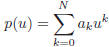
that solves the approximation problem
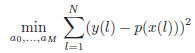
That is, the graph of the polynomial p(u) has to best
approximate the graph of the data pairs (x(k),y(k)) in the
least mean squares sense. The general syntax
of polyfit is:
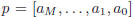
>>p=polyfit(x,y,M)
where, in the notations of (7), we identify “p” with the
coefficients’ vector  .
.
*The MATLAB function
polyval is used to evaluate a polynomial v=p(u) at a
point, or list of points x. The syntax is
>>y=polyval(p,x)
where the interpretation of
 is as
above, and where x is a single variable or an array. The returned value(s) y=p(x) are stored in an array y whose size is the same
size as that of x.
is as
above, and where x is a single variable or an array. The returned value(s) y=p(x) are stored in an array y whose size is the same
size as that of x.
5.5 Linear Fitting of The Speed of Sound Experiment
As stated above, our goal is to fit the data pairs (ttime,tdistance)
by a straight line, as in (6). You should therefore include in your M-file the command
>>est=polyfit(ttime,tdistance,1)
In accordancewith the notations of (6), the returned vectorwill
be the best estimate of est=[est(1),est(2)]=[speed of sound, bias]. If we want to see how good this estimate is, we
should substitute the estimated coefficients and the entries of ttime in the right hand side of (3). This is done
with the command
>>polyval(est,ttime)
For a visual comparison you will therefore include in your
program a plot command that compares the raw data with the linear estimate
>>plot(ttime,tdistance,’k*’,ttime,polyval(est,ttime))
Notice that here we allow a continuous plot of the linear
approximation . Add a title (including name of team members) and axes labels commands.
To evaluate the quality of your estimate of the speed of sound,
search the web for “speed of sound” and compare your estimate to what you find in the web. The site http://hyperphysics.phy-astr.gsu.edu/hbase/sound/souspe.html
is one option.
5.6 Acoustic Distance Measurement
Here you will compute the estimated distance from the
transducers to the clipboard in the experiments carried in §4. The estimated distance is given by Equation 5, where you have to use
your estimates of the speed of sound and the bias term. That is, you have to use theMATLAB function polyval and the
linear polynomial est=[est(1),est(2)]=[speed of sound, bias]. In your report compare the distance estimate
with the actual distance, as recorded in the experiment.
6 An Alternative model
As an alternative to the model (3), you will seek a
representation of the distance as a function of the maximal peak-to-peak amplitude of the receiver signal. We expect a reverse relation:
the longer the distance, the smaller the amplitude. Therefore the sought model
will be a function of the variable
 . You are allowed to use the polyfit function to test polynomial approximations of the form
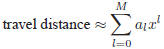
with various levels of the degree M. At this point you may rely
on visual inspection to evaluate the quality of the approximation. Clearly, the higher the degree M you allow, the
better the fit can be. However, we want the simplest possible formula, and will stop increasing M if there is no
noticeable improvement. The findings in your report should include:
• The values of the optimal coefficients and polynomial degree
• A plot, comparing the discrete data pairs ttime,amplitude with
the plot of the approximating function (9) that you identified. The plot must include a title (with your name)
and axes labels.
Hint: To create the data vector
from the data vector amplitude, you use the
place-by-place vector division command
>> x=1./amplitude;
If you expect the amplitude to vary with the distance according
to a power law , (amplitude = constant * distancen) you can try another way to fit the data: Taking the logarithm of
both sides of the equation above, you get the following equation:
>>log (amplitude) = log (constant) + n log(distance)
If you then define new variables:
u=log(amplitude)
v=log(distance)
L=log(constant)
you get the equation:
u = L + n * v
This is a linear equation and you can do a least squares fit to
the data to get he best fit value for n ( the slope ) and L (the y-intercept). Using the data you took for amplitude vs.
distance, use MATLAB to create the new variables u and v. Then use polyfit to get the best fit values for the slope and y
intercept . Finally, convert your results back to get the best fit values for
constant and n in the equation above: amplitude = constant * distancen.
Question (answer in your lab report):
1. How does your best fit values for constant and n compare with
the values from your Power Law fit in Excel?
2. How do you think that Excel gets its Power Law fit?
3. How could you use polyfit and a linear straight line fit to
find the best fit values of yo and a from (x, y) data that fits the following exponential equation:
y = y_o * exp (a *x)