Consider solving the linear system
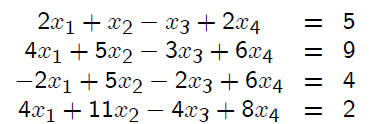
by Gaussian elimination without pivoting. We denote
this linear system by Ax = b. The augmented matrix
for this system is
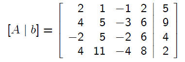
To eliminate x1 from equations 2, 3, and 4, use multipliers

To eliminate x1 from equations 2, 3, and 4, use multipliers

This will introduce zeros into the positions below the
diagonal in column 1, yielding
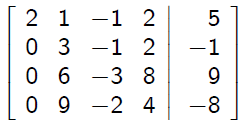
To eliminate x2 from equations 3 and 4, use multipliers

This reduces the augmented matrix to
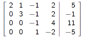
To eliminate x3 from equation 4, use the multiplier

This reduces the augmented matrix to
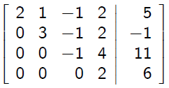
Return this to the familiar linear system
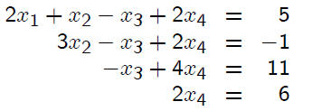
Solving by back substitution , we obtain

There is a surprising result involving matrices associated
with this elimination process. Introduce the
upper triangular matrix
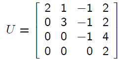
which resulted from the elimination process. Then
introduce the lower triangular matrix

This uses the multipliers introduced in the elimination
process. Then

In general, when the process of Gaussian elimination
without pivoting is applied to solving a linear system
Ax = b, we obtain A = LU with L and U constructed
as above.
For the case in which partial pivoting is used, we obtain
the slightly modified result
LU = P A
where L and U are constructed as before and P is a
permutation matrix. For example, consider
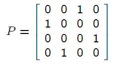
Then

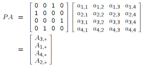
The matrix P A is obtained from A by switching around
rows of A. The result LU = P A means that the LU -
factorization is valid for the matrix A with its rows
suitably permuted
Consequences: If we have a factorization
A = LU
with L lower triangular and U upper triangular, then
we can solve the linear system Ax = b in a relatively
straightforward way.
The linear system can be written as
LU x = b
Write this as a two stage process:
Lg = b, U x = g
The system Lg = b is a lower triangular system
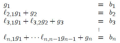
We solve it by “forward substitution”. Then we solve
the upper triangular system U x = g by back substitution.
VARIANTS OF GAUSSIAN ELIMINATION
If no partial pivoting is needed, then we can look for
a factorization
A = LU
without going thru the Gaussian elimination process.
For example, suppose A is 4 × 4. We write
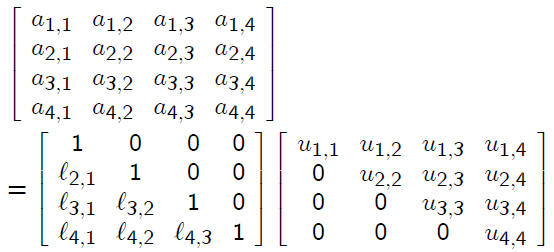
To find the elements ,
we multiply
the right side matrices L and U and match the results
with the corresponding elements in A.
Multiplying the first row of L times all of the columns
of U leads to

Then multiplying rows 2, 3, 4 times the first column
of U yields

and we can solve for .
We can continue
this process, finding the second row of U and
then the second column of L, and so on. For example,
to solve for
 ,
we need to solve for it in

Why do this? A hint of an answer is given by this
last equation. If we had an n × n matrix A, then we
would find
 by solving for it in the equation

Embedded in this formula we have a dot product. This
is in fact typical of this process, with the length of the
inner products varying from one position to another.
Recalling §2.4 and the discussion of dot products, we
can evaluate this last formula by using a higher precision
arithmetic and thus avoid many rounding errors.
This leads to a variant of Gaussian elimination
in which there are far fewer rounding errors.
With ordinary Gaussian elimination, the number of
rounding errors is proportional to n ^3. This reduces
the number of rounding errors, with the number now
being proportional to only n^2. This can lead to major
increases in accuracy, especially for matrices A which
are very sensitive to small changes.
TRIDIAGONAL MATRICES
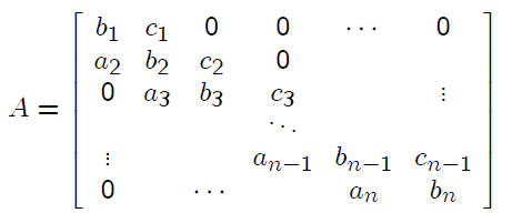
These occur very commonly in the numerical solution
of partial differential equations , as well as in other applications
(e.g. computing interpolating cubic spline
functions).
We factor A = LU , as before. But now L and U
take very simple forms . Before proceeding, we note
with an example that the same may not be true of the
matrix inverse.
EXAMPLE
Define an n × n tridiagonal matrix
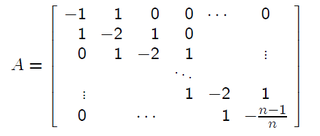
Then A−1 is given by

Thus the sparse matrix A can (and usually does) have
a dense inverse.
We factor A = LU, with
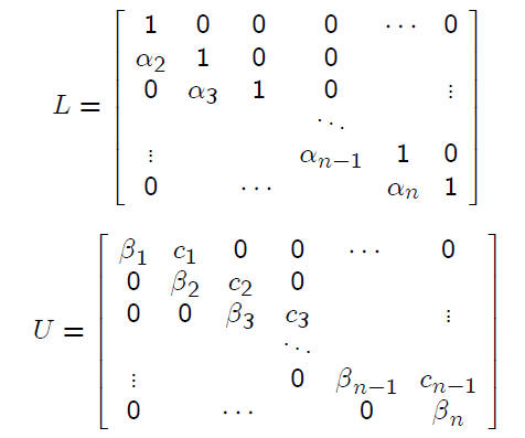
Multiply these and match coefficients with A to find

By doing a few multiplications of rows of L times
columns of U , we obtain the general pattern as follows.

These are straightforward to solve.

To solve the linear system
Ax = f
or
LU x = f
instead solve the two triangular systems
Lg = f, U x = g
Solving Lg = f :

Solving U x = g:

See the numerical example on page 278.
OPERATIONS COUNT
Factoring A = LU .
Additions : n − 1
Multiplications: n − 1
Divisions : n − 1
Solving Lz = f and U x = z:
Additions: 2n − 2
Multiplications: 2n − 2
Divisions: n
Thus the total number of arithmetic operations is approximately
3n to factor A; and it takes about 5n to
solve the linear system using the factorization of A.
If we had A−1 at no cost, what would it cost to compute
x = A−1f?

MATLAB MATRIX OPERATIONS
To obtain the LU-factorization of a matrix, including
the use of partial pivoting, use the Matlab command
lu. In particular,
[L, U, P] = lu(X)
returns the lower triangular matrix L, upper triangular
matrix U , and permutation matrix P so that
P X = LU


