Princeton University MATH 202

• Remind students that Adrian Banner’s review sessions starts this week: Tuesdays 7:30pm -
9:30pm in Fine 314

• Motivation: recall Linear Combination . First chapter: given a matrix A and a vector b, want
to know the vector x such that Ax = b... or, whether b is a linear combination of the column
vectors of A. Now we want to think about the case where we are given some pairs (x, b)
and see how we can find an A that transforms x into b.

• The topic is Linear Transformations

– A transformation T from a set X to a set Y is a rule that assigns to every x ∈ X an element
y = T(x) ∈ Y . We call the set X the domain or the source of the transformation,
and the set Y the co-domain or the target of the transformation.

– To express that T is a transformation from X to Y , we write

T : X → Y

– To expression that T takes an element x to an element y, we write

T(x) = y

or, sometimes we drop the parenthesis and write

Tx = y

We call y the image of x under T.

– ( Draw picture .)

– If the set X is for some whole number M , and the set Y is for some N, then in
both of the spaces we have the concept of lines and the concept of the origin (the point
(0, 0, . . . , 0)). If a transformation

is such that the image of any line is still a line, and the image of the origin is still the
origin, then we say that the transformation T is linear.

– Above is a geometric definition. It says that essentially, a linear transformation is
one that preserves the concept of lines and the concept of the origin. The geometric
concept of lines in is the same as the algebraic concept of addition of vectors . The
geometric concept of an origin is the same as the algebraic concept of multiplication
by a scalar number. So we can equivalently say that a linear transformation is one that
preserves the concept of vector-addition and the concept of multiplication of a vector
by a scalar number.

– So the equivalent definition for a linear transformation is that given
  two vectors in , and k a scalar, that T satisfies

And this is the definition that we will use.

– Examples:

* The transformation T : R → R given by T(x) = x² is NOT linear. Since

4 = T(2) = T(1 + 1) ≠ T(1) + T(1) = 1 + 1 = 2

Notice that for a transformation, not every element in the co-domain can be written
as the image of an element in the domain: the negative numbers in R cannot be the
image of this T. The subset of the elements in the co-domain which are images of
elements in the domain is called the range of the transformation.

* The transformation T : R² → R given by

is not linear. We can check this in several ways. The geometric definition requires
that the image of the origin be the origin. The origin in R² is and the origin in
R is just 0. But

so T is not linear. You can also check that this is not linear by explicitly showing
that

* Let T : R → R³ be

then T is linear. As we can check that

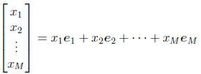
• Remember we talked about a linear combination of vectors last week. So now let’s do
something that looks a little bit stupid: we write

• In general, we can write

where

with the “1” in the ith row. We call the e_i’s the standard vectors in .

• What’s the point of splitting up a perfectly good vector into bits, you ask. The answer is
so we can better understand the linear transformation of a vector. Suppose we are given a
vector . We are interested in knowing how it transforms
under T. Using the definition of linearity, we know that

Does this not look awfully familiar?

• Yes, the expression looks just like the first method of multiplying a vector to a matrix. Recall
that we can write a N × M matrix as M separate column vectors, each of size N, stacked
next to each other, so that the matrix . Then we we multiply A by the
vector x, we end up with

• So the punch-line, every linear transformation



can be written as an N × M matrix. In particular, given the standard vectors of , we
can write the matrix A corresponding to T as



i.e., the matrix A corresponding to a linear transformation T is formed by stacked the size-N
column vectors corresponding to the images of the standard vectors next to each other.

• Now, remember that multiplication of a matrix by a vector is also linear in the sense that

A · (x + ky) = Ax + kAy

we see that the transformation from to given by the multiplication of an N × M
matrix is naturally a linear transformation.

• So.... we have another equivalent definition of a linear transformation: T is a linear transformation
from to if and only if the transformation can be written as a multiplication
by an N × M matrix. We will use this definition and the linearity definition above interchangeably.

• Examples

– Let a, b, c, d be the points in R² given by (1, 1), (1,−1), (−1,−1), (−1, 1). Is the transformation
T : R² → R² which satisfies

Ta = b, Tc = a, Tb = d, Td = c

a linear map? The answer is no. Notice that a = −c = (−1)c. But

Ta = b ≠ −a(= c =)(−1)Tc

So T is not linear.

– Given a vector w in . The transformation from → R given by

T(x) = w · x

where the two multiplies by the dot product is a linear transformation. That is because
of our second method of multiplying matrix against vectors: w · x can be written as
multiplying the vector x to a 1 ×M matrix whose ith column is the ith entry of w.

– The projection

from R³ → R² is linear, and its corresponding 2 × 3 matrix is

– Another linear map is

Its matrix is

– The map T : → give by

T(x) = x

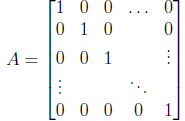
is called the identity transformation. Its corresponding matrix is

with 1s on the diagonal and 0s everywhere else. This matrix comes up often enough
that we’ll give it a name: it is called the identity matrix on and is written I_M.