Functions

§1. Entering and Storing Functions
§2. Vector-Valued Functions
§3. Composition of Functions and Inverse Functions
§4. Trigonometric Functions

Function is a data type in the TI-89. There are many things that we can do with certain
functions. This is loosely coordinated with Chapter 2 of the text Calculus with Early Vectors, by
Phillip Zenor, Edward Slaminka, and Donald Thaxton, Prentice Hall , 1999.

1. Entering and Storing Functions

In the Home screen we can store a formula for a function using the Define command or the
STO key. We can use any variable name (up to eight characters beginning with a letter) as the
name for the function.

Custom menu items

Notice in the first row of figures that we define a function f(x), which we can evaluate using
function notation. In the second row of figures, we name an expression instead. To evaluate an
expression, use the vertical bar to temporarily assign a value to x. Pressing the VAR-LINK
keystroke brings up a list of all the variables defined, the data type, and the bytes of storage
required. While a variable in the VAR-LINK list is highlighted, you can press F6 Contents to
see one screen of the definition or program (which is usually enough to remember what you have
stored here). If you press ENTER while the name is highlighted, the name will be pasted into the
command line. If you press the destructive back arrow while the name is highlighted, you can
delete the object from memory.

You can store a formula in the Y= Editor in the three ways demonstrated above. All three
functions will end up showing in the Y= Editor screen and will be selected (with the check mark)
since they are new. Again, I highly recommend that you look at a table of values for these
functions before trying to select a viewing window.

2. Vector-Valued Functions

In the Home screen, we can define a vector-valued function.

Since the output of such a vector-valued function on the TI-89 is a matrix, we cannot use such a
function on one of the function slots of the Y= Editor. We can plot each component function
separately. Notice below that in Function graphing, the graphing variable must be x.

For functions from R to R² , we can use Parametric graphing to show the image (not the graph
which would require three dimensions). In Parametric graphing, the graphing variable is t.

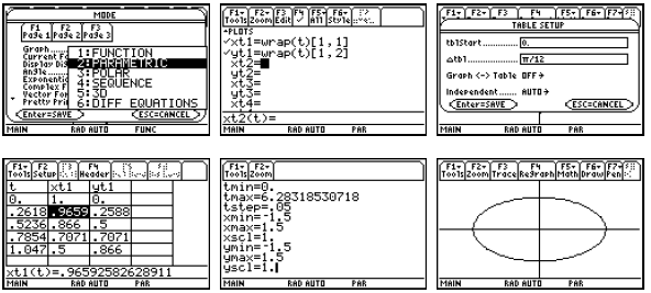
Often when plotting a two-dimensional image, we might be happier using a plot with equallyscaled
axes. The F2 Zoom 5:ZoomSqr command will widen the range of either the x-axis or the
y-axis so that we see everything we saw before only in window with equally-scaled axes. Then
this plot will look like a circle .

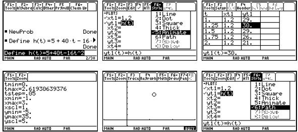
We can also use parametric graphing to simulate some motion problems. Suppose that
h(t) = 5 + 40t −16t² describes the height of a ball (in feet) thrown straight up at time t = 0 after t
seconds. We can provide an animation of the motion, the image of h, and the graph of h. Notice
we have set tmax below to correspond with the time when the ball hits the ground.

3. Composition of Functions and Inverse Functions

There is no special symbol for the composition f o g , but it can be accomplished via f (g(x))
in the Home screen. Where possible, the result will be simplified.

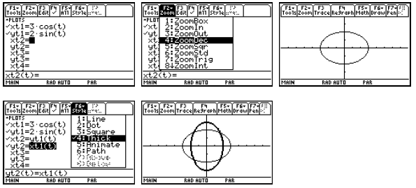
For any relation (or equation) of two variables , we can define the inverse relation to be what you
get when you interchange x and y. For example the equation gives a plot
which is an ellipse . The inverse relation gives the plot
. We can get the first relation on the calculator with the parametric
equations x = 3cos t and y = 2sin t , 0 ≤ t ≤ 2π . We can also plot the inverse relation by
switching the parametric equations. Since x and y have been interchanged, the second plot we
get is the reflection about the line y = x of the first plot.

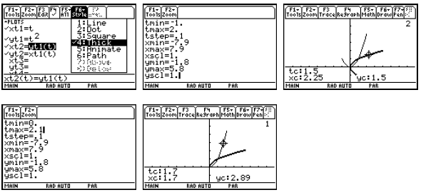
For any real -valued function f(t), plotting the parametric equations x = t and y = f(t) gives the
graph of the function f, and plotting x = f(t) and y = t gives the graph of the inverse relation.
When the function f happens to be one-to-one and have an inverse function f ⁻¹ , the plot of the
inverse relation will actually be the graph of the inverse function. In Parametric graphing, we
may be able to restrict the domain (via the choice of tmin and tmax) in order to make the plot
one-to-one. Notice that you can trace on either curve .

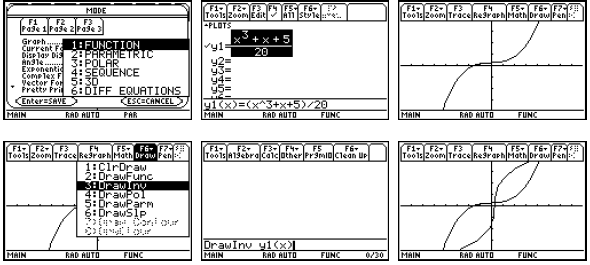
In Function graphing mode, the calculator provides a command to have the inverse relation as a
“drawn” object. However “drawn” objects cannot be traced, and they disappear when the graph
is re-plotted for any reason. It is also hard to restrict the domain in Function graphing mode.

For very simple functions (little more than linear polynomials), the solve command in the Home
screen can enable us to find the formula for the inverse function.

4. Trigonometric Functions

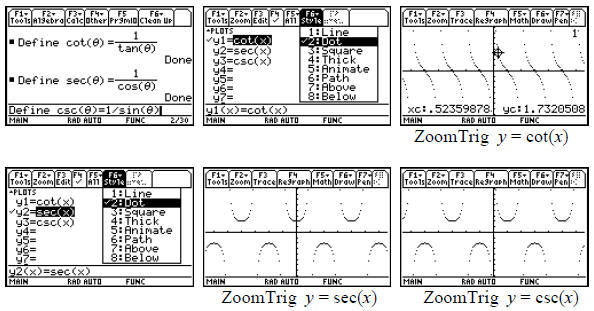
The calculator provides the trigonometric functions for the sine, cosine, and tangent. It also
provides an inverse function for each (on a suitably restricted domain). The other trigonometric
function can be computed from these, but it might be nice to have them defined permanently. If
we use variable names longer than one letter, then the commands in the F6 Clean Up menu like
NewProb will not delete these functions.

we use variable names longer than one letter, then the commands in the F6 Clean Up menu like
NewProb will not delete these functions.

We can also compute the inverse functions for the cotangent, secant, and cosecant functions in
terms of the inverse trigonometric functions provided. There is simply a question of the most
desirable domain and range. For example, if we desire the inverse cotangent, we consider the
following algebra .

implying that

Most people do not like this choice of range for the inverse cotangent (and it leaves the problem
of what to do with

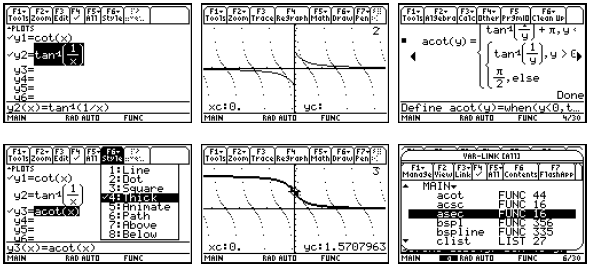
As in many computer languages, we use “acot” as the variable name for the inverse cotangent or
arccotangent, and then “asec” and “acsc” for the remaining inverse functions. Make the
following definitions to have these functions.

Define
Define
Define

When you want to use these functions, you can either type the name or you can get it from your
VAR-LINK list of all of your variables as in the last figure above.

By the way, all of the above steps are not needed if you will simply upgrade your OS to at least
version 2.08 where the “other” trigonometric functions and their inverses have been included.
Since the variable names “cot”, “sec”, and “csc” become reserved words in the newer versions of
the operating system , you will not be allowed to keep programs around with these names.