Introduction We will discuss different ways to
discuss differences in prportions between treatments
or populations. We will use this to develop stratification and modeling.
Taxonomy of Studies
Retrospective or case-control study: select cases, select controls,
compare exposure
Prospective study: select exposed cases, and controls not exposed.
Compare incidences after
some time.
Cross-sectional study: select a sample without regard to disease or risk
factor, then divide
according to exposure. Compare prevalence .
Randomized study: select a sample, randomize to treatment or control,
then compare.
Prospective, cross-sectional and randomized studies can be
analyzed similarly.
Retrospective studies require extra caution.
Independence in Probability and Statistics
Observations are statistically independent if knowing
the value of one observation tells you nothing about any of the others.
The formal statistical definition is that events A and B are independent if
P(A and B) = P(A)P(B)
or, in terms of statistical probability density functions,
if the joint density function is the product
of the marginal density functions:
f(x, y) = f(x)f(y), for all x and y
If observations are statistically independent, the
variance of their sum equals the sum of the variance;
this is used to calculate the standard deviation of the mean.
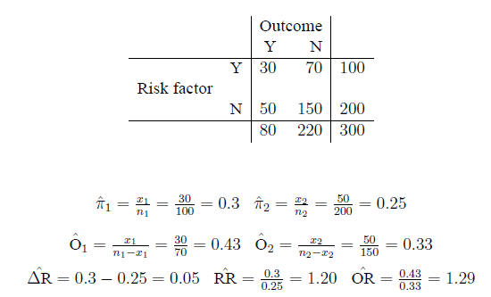
Contingency tables A contingency table is a
standard layout for comparing events in two populations:

Probability, risk and odds Probability: the
fraction of times an event is expected to occur in a
population of size N

is estimated by the fraction of times it occurs in a
sample of size n:

Risk is a term used interchangably with probability
(assuming events are undesirable)

The odds of an event equal the probability an event
occurs, divided by the probability it does not:

The relationship between odds and probability is
straightforward:

There are three measures for comparing the difference
between two proportions:
Arithmetic difference
Relative risk
Odds ratio
Arithmetic difference Difference in risk:
arithmetical difference (rather than the ratio) of two
probabilities:

Relative risk The ratio of probabilities in two
homogeneous populations

is estimated by the ratio of probabilities in two samples:

The hazard ratio is similar to the relative risk, but is
used in connection with survival studies where
there are censored data
Odds ratio The odds ratio between two populations
is just like it sounds:

and is estimated from the sample in the expected fashion:

Example Example:

Confidence intervals for the arithmetic difference
Proportion of successes (events) in each
group:

The standard error of the difference
 is:
is:

95% Confidence interval for

In the example,

so

Confidence interval for the relative risk The
relative risk does not have a Gaussian distribution
on the original scale, but its logarithm is approximately Gaussian.
Calculate

Then

In the example,

Confidence interval for the odds ratio The
distribution of the odds ratio is not symmetric
Calculate

Then

In the example,

Differences between proportions and ratios When do
you study the arithmetic difference between
two proportions , and when do you study the ratio between two proportions?
Use whichever makes contextual sense, e.g.:
What is the scientific significance of an increase of 1%?
What is the scientific significance of an increase of a doubling of risk?
Note that the test for the difference between two means
doesn’t work well if either proportion is
very close to 0 or 1.
Retrospective Trials versus Ecerything Else In a
prospective, cross-sectional or experimental
study, populations are sampled so that the only the grand total or the marginal
row totals of the
contingency table are fixed, and risk information is preserved.
In a retrospective case-control study, the column
marginals, rather than the row marginals of the
contingency table, are set by experimental design.
The odds ratio is more appropriate for case-control
studies. The relative risk cannot be calculated
because there is no information about risk or incidence in the data; the
relative proportion of cases
to controls is investigator-driven.
If the disease is fairly rare, the odds ratio is a good
approximation to the relative risk.
Stratified analysis is useful if the outcome varies
between the strata, and the strata can be identified
before analysis, preferably at the design stage
If you know a variable is going to affect the outcome,
it’s a good idea to stratify and randomize
within the strata
Generally, you need to state if you are going to do
separate within-strata analyses. If so, reviewers
may want to size each strata. 1 . Stratified analysis
Simple steps in controlling for confounding through
stratified analysis are:
Calculate the relative risk (RR) or odds ratio (OR, which
is an estimate of the RR) without
stratifying (crude RR or crude OR)
Stratify by the confounding variable
Calculate the adjusted RR (or OR)
Compare the crude RR or OR with the adjusted RR or OR
If the adjusted estimate (aRR or aOR) is equal to the
unadjusted one (RR or OR), then there is no
confounding. If they are different, then there is confounding. But one may ask,
how big should
the difference be? Rule of thumb : if the CRUDE RELATIVE RISK differs from the
ADJUSTED
RELATIVE RISK by 10% or more, there is important confounding. The adjusted RR
should then
be calculated by stratifying the confounding variable.
The 95% CI (and formal significance testing) can now be
carried out to measure the significance
of the association between the risk factor and the problem for the different
strata .
Note that, in order to deal with confounding variables,
they must be identified. The advantage of
randomization is that both identified and unidentified confounders are
distrubted among the test
and control groups .


