Polynomials in Matlab

Polynomials

•
• n is the degree of the polynomial
• Examples:
f(x) = 2x² - 4x + 10 degree 2
f(x) = 6 degree 0

Polynomials in Matlab

• Represented by a row vector in which the
elements are the coefficients.
• Must include all coefficients, even if 0
• Examples
8x + 5 p = [8 5]
6x² - 150 h = [6 0 -150]

Value of a Polynomial

• Recall that we can compute the value of a
polynomial for any value of x directly.
• Ex: f(x) = 5x³ + 6x² - 7x + 3

x = 2;
y = (5 * x ^ 3) + (6 * x ^ 2) - (7 * x) + 3
y =
53

• Matlab can also compute the value of a
polynomial at point x using a function,
which is sometimes more convenient
• polyval (p, x)
– p is a vector with the coefficients of the
polynomial
– x is a number, variable or expression

• Ex: f(x) = 5x³ + 6x² - 7x + 3
p = [5 6 -7 3];
x = 2;
y = polyval(p, x)
y =
53

Roots of a
Polynomial

• Recall that the roots of a polynomial are
the values of the argument for which the
polynomial is equal to zero
• Ex: f(x) = x² - 2x -3
0 = x² - 2x -3
0 = (x + 1)(x - 3)
0 = x + 1 OR 0 = x - 3
x = -1
x = 3

• Matlab can compute the roots of a function
• r = roots(p)
– p is a row vector with the coefficients of the
polynomial
– r is a column vector with the roots of the
polynomial

• Ex: f(x) = x² - 2x -3
p = [1 -2 -3];
r = roots(p)
r =
3.0000
-1.0000

Polynomial
Coefficients

• Given the roots of a polynomial, the
polynomial itself can be calculated
• Ex: roots = -3, +2
x = -3 OR x = 2
0 = x + 3
0 = x - 2
0 = (x + 3)(x - 2)
f(x) = x² + x - 6

• Given the roots of a polynomial, Matlab
can compute the coefficients
• p = poly(r)
– r is a row or column vector with the roots of
the polynomial
– p is a row vector with the coefficients

• Ex: roots = -3, +2
r = [-3 +2];
p = poly(r)
p =
1 1 -6
% f(x) = x² + x -6

Adding and Subtracting
Polynomials

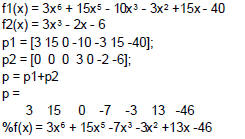
• Polynomials can be added or subtracted
• Ex: f1(x) + f2(x)

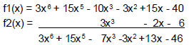
• Can do this in Matlab by just adding or
subtracting the coefficient vectors
– Both vectors must be of the same size, so the
shorter vector must be padded with zeros

Ex:

Multiplying Polynomials

• Polynomials can be multiplied:
• Ex: (2x² + x -3) * (x + 1) =

• Matlab can also multiply polynomials
• c = conv(a, b)
– a and b are the vectors of the coefficients of
the functions being multiplied
– c is the vector of the coefficients of the
product

• Ex: (2x² + x -3) * (x + 1)
a = [2 1 -3];
b = [1 1];
c = conv(a, b)
c =
2 3 -2 -3
% 2x³ + 3x² -2x -3

Dividing Polynomials

• Recall that polynomials can also be
divided

• Matlab can also divide polynomials
• [q,r] = deconv(u, v)
– u is the coefficient vector of the numerator
– v is the coefficient vector of the denominator
– q is the coefficient vector of the quotient
– r is the coefficient vector of the remainder

• Ex: (x² - 9x -10) ÷ (x + 1)
u = [1 -9 -10];
v = [1 1];
[q, r] = deconv(u, v)
q =
1 -10 % quotient is (x - 10)
r =
0 0 0 % remainder is 0

Example 1

• Write a program to calculate when an object
thrown straight up will hit the ground. The
equation is
s (t) = -½gt² +v₀t + h₀
s is the position at time t (a position of zero
means that the object has hit the ground)
g is the acceleration of gravity: 9.8m/s²
v₀ is the initial velocity in m/s
h₀is the initial height in meters (ground level is 0,
a positive height means that the object was
thrown from a raised platform)

Prompt for and read in initial velocity
Prompt for and read in initial height
Find the roots of the equation
Solution is the positive root
Display solution

v = input('Please enter initial velocity: ');
h = input('Please enter initial height: ');
x = [-4.9 v h];
y = roots(x);
if y(1) >= 0
fprintf('The object will hit the ground in %.2f seconds \n',
y(1))
else
fprintf('The object will hit the ground in %.2f seconds \n',
y(2))
end

Please enter initial velocity: 19.6
Please enter initial height: 58.8
The object will hit the ground in 6.00
seconds

• We can take the derivative of polynomials
f(x) = 3x² -2x + 4
dy = 6x - 2
dx

• Matlab can also calculate the derivatives
of polynomials
• k = polyder(p)
p is the coefficient vector of the polynomial
k is the coefficient vector of the derivative

• Ex: f(x) = 3x² - 2x + 4
p = [3 -2 4];
k = polyder(p)
k =
6 -2
% dy/dx = 6x - 2

• ?6x² dx = 6 ?x² dx
= 6 * ? x³
= 2 x³

• Matlab can also calculate the integral of a
polynomial
g = polyint(h, k)
h is the coefficient vector of the polynomial
g is the coefficient vector of the integral
k is the constant of integration - assumed
to be 0 if not present

• ?6x² dx
h = [6 0 0];
g = polyint(h)
g =
2 0 0 0
% g(x) = 2x³

Polynomial Curve Fitting

• Curve fitting is fitting a function to a set of
data points
• That function can then be used for various
mathematical analyses
• Curve fitting can be tricky, as there are
many possible functions and coefficients

Curve Fitting

• Polynomial curve fitting uses the method
of least squares
– Determine the difference between each data
point and the point on the curve being fitted,
called the residual
– Minimize the sum of the squares of all of the
residuals to determine the best fit

• A best-fit curve may not pass through any
actual data points
• A high- order polynomial may pass through
all the points, but the line may deviate
from the trend of the data

Matlab Curve Fitting

• Matlab provides an excellent polynomial
curve fitting interface
• First, plot the data that you want to fit
t = [0.0 0.5 1.0 1.5 2.0 2.5 3.0 3.5 4.0 4.5 5.0];
w = [6.00 4.83 3.70 3.15 2.41 1.83 1.49 1.21 0.96 0.73
0.64];
plot(t, w)
• Choose Tools/Basic Fitting from the menu
on the top of the plot

• Choose a fit
– it will be displayed on the plot
– the numerical results will show the equation
and the coefficients
– the norm of residuals is a measure of the
quality of the fit. A smaller residual is a better
fit.
• Repeat until you find the curve with the
best fit

Linear Fit

8th Degree Polynomial

Example 2

• Find the parabola that best fits the data
points (-1, 10) (0, 6) (1, 2) (2, 1) (3, 0)
(4, 2) (5, 4) and (6, 7)
• The equation for a parabola is
f(x) = ax² + bx + a

X = [-1, 0, 1, 2, 3, 4, 5, 6];
Y= [10, 6, 2, 1, 0, 2, 4, 7];
plot (X, Y)

Other curves

• All previous examples use polynomial
curves. However, the best fit curve may
also be power , exponential, logarithmic or
reciprocal
• See your textbook for information on fitting
data to these types of curves

Interpolation

• Interpolation is estimating values between
data points
• Simplest way is to assume a line between
each pair of points
• Can also assume a quadratic or cubic
polynomial curve connects each pair of
points

• yi = interp1(x, y, xi, 'method')
interp1 - last character is one
x is vector with x points
y is a vector with y points
xi is the x coordinate of the point to be
interpolated
yi is the y coordinate of the point being
interpolated

• method is optional:
'nearest' - returns y value of the data point that
is nearest to the interpolated x point
'linear' - assume linear curve between each two
points (default)
'spline' - assumes a cubic curve between each
two points

• Example:
x = [0 1 2 3 4 5];
y = [1.0 -0.6 -1.4 3.2 -0.7 -6.4];
yi = interp1(x, y, 1.5, 'linear')
yi =
-1
yj = interp1(x, y, 1.5, 'spline')
yj =
-1.7817