1. 2.1.1 Fixed points are points where sinx = 0, that is,
integer multiples of π.
2.1.2 The greatest velocity to the right occurs where sinx
is the greatest. That is, where x is π/2
plus an integer multiple of 2π.
2.1.3 a) implies
 by the chain rule , so
 Did you
remember that cosxsinx = sin(2x)/2? If not, here is an easy way to memorize it:
Among the
trigonometric formulas , the only ones that I memorize are sin(a+b) =
sinacosb+cosasinb
and cos(a+b)=cosacosb−sinasinb. All others follow from these very quickly. For
example,
the first with a = b = x gives you what you need for this problem. b) The
acceleration to the
right is greatest where sin(2x) is greatest, that is where x = π/4 plus an
integer multiple of π.
2. 2.2.1. Sketch of the vector field:
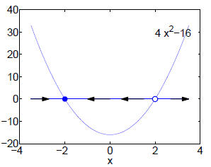
x = −2 is a stable fixed point, and x = 2 is unstable, as
is apparent from the vector field.
Here is what the solutions look like:
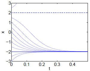
(Solutions with x > 2 blow up in finite time.)
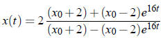
Solution in closed form: If then x(t) = ±2 for
all t, since 2 and −2 are fixed points.
then x(t) = ±2 for
all t, since 2 and −2 are fixed points.
Let’s assume that
 now. Then x(t) ≠ ±2 for all t (this is true by the uniqueness part of
the existence and uniqueness theorem). This will be used in the following
manipulations.
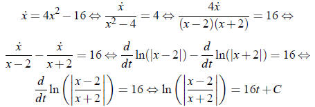
for some constant C, which is found by plugging in t = 0.
Using the notation  we find
So
Exponentiate both sides of this equation:
So
For t = 0, the correct sign is +. Therefore the correct
sign must be + for all t. (If the sign
changed from + to − all of the sudden, x would have to be discontinuous at that
point!) So
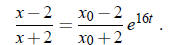
Multiply this equation by x +2, then solve for x :
3. 2.2.8 It is best to draw a suitable function first:
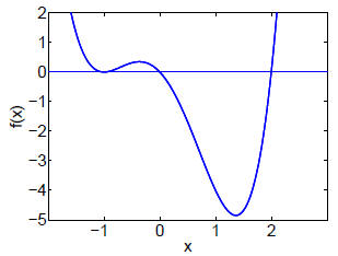
After that, it’s almost as easy to write down a formula defining a function that
looks like that,
qualitatively:
f (x) = x(x+1)2(x−2)
(In fact, the above plot shows precisely that function.)
2.2.9 The function must vanish ( be zero ) at x = 0 and x =
1. It must be negative between 0 and
1, and positive everywhere else. Its minimum must occur near x = 1/2. It must
increase for
x > 1, and decrease for x < 0. (Can you see why?) A function that meets all
these criteria is
f (x) = x(x−1) .
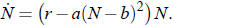
4. 2.3.4 To motivate this problem, suppose that in general

describes population growth. We certainly want
f (0) = 0.
This just expresses the fact that it is possible that there is no population at
all, and never will be.
Now what are the simplest choices of functions f = f (N) with f (0)= 0? The very
simplest
one is linear :
f (N) = rN.
This gives rise to exponential growth (or, if r < 0, decay). The second-simplest
is quadratic:
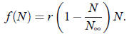
This gives rise to logistic growth , as we discussed in class;
 is the carrying
capacity. (The
is the carrying
capacity. (The
physically interesting case is r > 0. What happens if r < 0?) This problem is
about the third-simplest
case, that of a cubic function f . Since f (0) is to be zero, we must be able to
write f (N)
as N times a quadratic function. Strogatz writes it like this:
f (N) = (r−a(N−b)2) N
 (1)
(1)
Any quadratic function can be written in the form r −a(N −b)2. So our population
growth
equation is then.
 (2)
(2)
Let us first consider the case when N = 0 is the only fixed point, that is, when
the equation
r−a(N −b)2 = 0 (3)
has no solution. One case in which Eq. (3) has no solution is a = 0, r
≠ 0. In
that case, Eq. (2)
becomes

the exponential growth (or, if r < 0, decay) model. This is not of interest to
us here, so let us
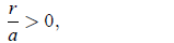
assume a ≠ 0. In that case, Eq. (3) has no solution if and only if
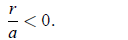 (4)
(4)
There are two possibilities: Either N = 0 is a stable fixed point, or an
unstable one. Which of
these two cases we are in depends on the sign of f ′(0). In general,
f ′(N) = r−a(N −b)2−2a(N −b)N,
and therefore
f ′(0) = r−ab2.
So N = 0 is stable if r < ab2, and unstable if r > ab2. Remember that we assume
(4), that is, we
assume that r and a are of opposite signs. Therefore if a > 0, then certainly r
< ab2, since then
r is negative and ab2 is positive. On the other hand, if a < 0, then certainly r
> ab2, since then
r is positive and ab2 is negative. This argument shows that in fact, if (3) has
no solution, then
N = 0 is a stable fixed point if a > 0, and an unstable one if a < 0. We could
have seen this by
a different argument as well: For large N,
( compare Eq . (1). Therefore, if a < 0, then f (N) → −∞ as N → −∞, and f (N) → +∞ as
N →+∞. If f crosses through N = 0 only once, it must cross from negative values
(for N < 0)
to positive ones (for N > 0), and therefore N = 0 must be unstable. One sees by
a precisely
analogous argument that N = 0 must be a stable fixed point if Eq. (3) has no
solution, and
a > 0.
But if N = 0 is the only fixed point, and is stable, the problem is
uninteresting: The population
simply goes extinct, no matter where we start. If N = 0 is the only fixed point,
and it
is unstable, then in fact Eq. (2) is unphysical, since it predicts blowup of the
population size in
finite time. (Do you see why?)
So we have now concluded that the case in which Eq. (3) has no solution is
uninteresting.
We will now assume
 (5)
(5)
so that Eq. (3) has two solutions. Those two solutions are
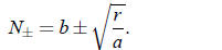 (6)
(6)
Either one of the two solutions of Eq. (3) could be zero, depending on the
parameter values,
but we will assume that they are not zero, so that there are three distinct
solutions of f(N) = 0,
rather than a solution of multiplicity two at N = 0.
There are three cases to distinguish now:
 (7)
(7)
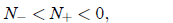
 (8)
(8)
and
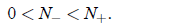 (9)
(9)
The negative fixed points are of no physical interest to us, so the number of
physically interesting
fixed points if one in case (7), two in case (8), and three in case (9). Case
(7) either leads to
guaranteed extinction of the population, if a > 0, or blowup in finite time, if
a < 0; the former
is uninteresting, the latter unphysical.
So let us proceed to case (8). Here there are again two possibilities. If a > 0,
the fixed
point 0 is unstable, and the fixed point  is stable. Therefore the population
will level off at
is stable. Therefore the population
will level off at
 for any initial value N (0) > 0. This is very similar to logistic growth, and
therefore not so
for any initial value N (0) > 0. This is very similar to logistic growth, and
therefore not so
interesting to us here. The other possibility is a< 0, in which case the
population will go extinct
if N(0) <  , and blow up in finite time if N(0) >
 — not a physical case.
So let us proceed to case (9). Again, we think about the two possibilities a > 0
and a < 0.
If a < 0, then the population will lever off to
 if 0 < N(0) <
 , and blow up
in finite time if
, and blow up
in finite time if
N(0)> —not a physical case. The only potentially interesting and physical case
is therefore
—not a physical case. The only potentially interesting and physical case
is therefore
that in which (9) holds and a > 0. In this case, the population will go extinct
if 0 < N(0) <  ,
,
and level off to  if N(0) >
 . Thus
  is an extinction threshold: If N(0) is
below it, the
is an extinction threshold: If N(0) is
below it, the
population goes extinct, if N(0) is above it, the population levels off to the
“carrying capacity”
 .
.
I summarize : The only choice of a cubic f which is interesting, physically
plausible, and
qualitatively different from exponential and logistic growth is that in which
a > 0, r > 0,

In this case, there are three fixed points, namely
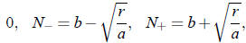
and
 is the extinction threshold, and N+ the carrying capacity.