In Signals and Systems , as well as other subjects in
Unified, it will often be necessary to solve systems of linear equations , such
as
x +2y +3z =1
2x +5y +2z =2
 (1)
(1)
x + y + z =3
There are are at least three ways to solve this set of
equations: Elimination of variables, Gaussian reduction, and Cramer’s rule.
These three approaches are discussed below.
Elimination of Variables
Elimination of variables is the method you learned in high school. In the
example, you first eliminate x from the second two equations, by subtracting
twice the first equation from the second, and subtracting the first equation
from the third. The three equations then become
x +2y +3z =1
y − 4z =0
 (2)
(2)
−y − 2z =2
Next, y is eliminated from the third equation, by adding
the (new) second equation to the third , yielding
x +2y +3z =1
y − 4z =0
 (3)
(3)
− 6z =2
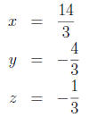
From the third equation, we conclude that
 (4)
(4)
From the second equation, we conclude that 4
 (5)
(5)
Finally, from the first equation, we find that
 (6)
(6)
Gaussian Reduction
A more organized way of solving the system of equations is
Gaussian reduction. First, the augmented matrix of the system is formed:
 (7)
(7)
Each row of the augmented matrix corresponds to one
equation in the system of equations. The first three elements of each row are
the coefficients of x, y, and z in the equation. The fourth element in each row
is the right-hand side of the corresponding equation.
The goal of the reduction process is to apply row
operations to the matrix to get zeros below the first diagonal of the matrix. To
do this for the example, subtract twice the first row from the second, and the
first row from the third, to obtain
 (8)
(8)
This produces zeros in the first column below the
diagonal. Then add the second row
to the third to obtain
 (9)
(9)
Normally, the process is stopped at this point, and “ back
substitution ” is used to solve for the variables. That is, the array above is
really the same as the last reduction we did in elimination of variables, so we
can proceed as before.
Alternatively, we could continue the process further, by
dividing the third row by -6, and then eliminating terms above the diagonal as
well, as follows:
 (10)
(10)
Subtract 3 times the third row from the first, and add 4
times the third row to the
second:
 (11)
(11)
Finally, subtract 2 times the second row from the first:
 (12)
(12)
from which we conclude that

as before.
There is really no need to repeatedly write down the
augmented matrix. Instead, it is convenient to write down the matrix with space
between the rows, and update a row at a time, crossing out the old row. (See
attached page.)
Note that the two methods , elimination of variables and
Gaussian reduction, are really the same approach. The only real difference is
that in Gaussian reduction, we don’t bother to write down x, y, and z. Instead,
the variables are associated with columns of the augmented matrix.
Cramer’s Rule
Cramer’s Rule is a method that is useful primarily for
low - order systems , with two or three unknowns. Cramer’s rules states that each
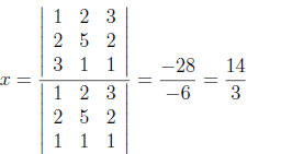
unknown can be expressed as the ratio of two matrix determinants. For example, x
(the first variable) is given
by
 (13)
(13)
The denominator is the determinant of the matrix of
coefficients of the equation, i.e.,

The numerator is the determinant of the same matrix,
except with the first column
replaced by the three numbers on the right-hand side of the equations. Likewise,
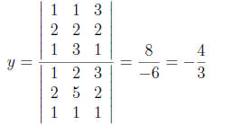
y is
found by a similar ratio, with the top matrix found by replacing the second
column
of the denominator matrix by the right-hand side column:
 (14)
(14)
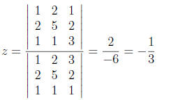
Finally,
 (15)
(15)
Cramer’s rule is very handy for second-and third-order
systems. However, it is much less useful for larger systems, because the
determinant calculation becomes prohibitive, if done in the conventional way.
(See section below.) Determinants can also be found by Gaussian reduction;
however, the reduction process does more than determine the determinant, it also
solves the equations! So just use Cramer’s rule for small “toy” problems.
Determinants
Finally, you need to know how to take determinants of
matrices. For second-order
matrices,
 (16)
(16)
For third-order systems,
 (17)
(17)
Both of these have an obvious pattern—each of the terms is
the product of diagonals, with a + sign for one direction of diagonal, and a −
sign for the other direction. Note that for the third-order case, the diagonals
“wrap around.”
For higher-order systems, there are two approaches to find
the determinant. One approach is to do Gaussian reduction to obtain a triangular
matrix. The determinant is then the product of the terms on the main diagonal.
The other approach is to decompose the determinant along,
say, the first row of the matrix. For each element A1j along the first row of
the matrix, find the matrix
formed by deleting the first row and jth column. Call the
determinant of that matrix dj . Then
 (18)
(18)
For example,
 (19)
(19)
Actually, we can expand on any row or column as above. When expanding on an
even-numbered row or column, the sign of the determinant is changed.
The only problem with the approach is that the amount of calculation required to
calculate the determinant using this approach goes like n!, but only goes like
n3 using Gaussian reduction. So it usually isn’t used for systems much higher
than third order.


