Basic Matrix Operations

1 Terminology

A matrix is a rectangular array of numbers, for example

,or

The numbers in any matrix are called its entries. The entries of a matrix are organized into rows and
columns, which are simply the horizontal and vertical (resp.) lists of entries appearing in the matrix. For
example, if

then the rows of M are and whereas the
columns of M are

,and .

It is worth noting that an m · n matrix will have m rows with n entries each, and n columns with m entries
each. That is, the number of entries in any row of a matrix is the number of columns of that matrix, and
vice versa. This is readily apparent in each of the examples above.

The dimensions of a matrix are the numbers of rows and columns it has. If a matrix has m rows and n
columns we say that it is an m · n matrix (note that we always list the number of rows first). So, the first
four matrices above have dimensions   and , respectively. The dimensions of the matrix
M are An m · n matrix is called square if m = n. Thus, the only example of a square matrix above
is the second.

So that we can more easily refer to various entries in matrices, we index the columns of a matrix from
left to right and the rows from top to bottom. For example, the first column of M (above) is

the second column is

the third column is

etc. The first row of M is the second row is and the third row is
We can use this numbering scheme to easily refer to entries in a matrix: we call the
entry located in row i and column j the i, j-entry. For the matrix

the 1, 1-entry is 1, the 3, 2-entry is -1, the 4, 3-entry is 9 and the 2, 1-entry is -1/6.

To write down a matrix with variable entries we use variables with subscripts that indicate their position
in the matrix, using the convention described above. A generic m· n matrix can therefore be denoted

or just   for short.
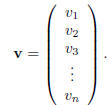
An m ·1 matrix has the form

and is called, appropriately, a column vector. Notice that since a column vector has only a single column we
have used only single subscripts to index its entries. Likewise, a 1· n matrix looks like

and is called a row vector. When we use the word vector with no qualification we will usually mean a column
vector. Column vectors give us another shorthand for writing down generic matrices. Notice that if we use
the matrix A in (1) and set

(i.e. we use the entries in the j-th column of A as the entries in a_j) then we can write

In a similar way one can also use the rows of A to express A in terms of row vectors, but since we won't be
using this idea later we won't bother to write it out.

2 Scalar multiplication and addition of matrices

Having dispensed with the basic terminology and notation of matrices, we now turn to how they are ma-
nipulated algebraically . We will see that it is possible to add, subtract and multiply matrices together, but
only if certain restrictions on their dimensions are met. We begin with the notion of scalar multiplication.
Given an m · n matrix A = (a_ij) and a number (scalar) c we define

That is, cA is the matrix obtained by multiplying every entry of A by c. As examples, if

then

Adding two matrices is also done entry-by-entry. If A = (a_ij) and B = (b_ij) are two m· n matrices, then
their sum is A + B = (a_ij +b_ij ). That is, the i, j-entry of A+ B is the sum of the i, j-entries of A and B. It
is important to note that is is only possible to add two matrices if they have exactly the same dimensions.
Here's an example: if

then

and

The following theorem summarizes the main · properties of matrix addition. The proofs of these properties
follow directly from the definitions made so far and are left to the reader. We will find it useful to be able
to refer to the m· n zero matrix , which is the matrix all of whose entries are zero.

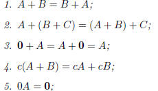
Theorem ·1. Let A, B and C be m· n matrices, let c be a real number and let 0 denote the m· n zero
matrix. Then

3 Matrix multiplication

Defining the matrix product is a two step process. First we will define what it means to multiply a matrix
by a column vector and then we'll use that to tell us how two multiply matrices in general. Let A be an
m ·n matrix and let v be an· n ·1 column vector (notice that the vector v has as many entries as A has
columns). Write A in terms of its columns as above,

and write out the entries of v as

The product of A with v is defined to be

In words, we multiply the columns of A by the respective entries of v and then add the results together.
According to this definition, the product of an m· n matrix and an· n ·1 column vector is an m ·1 column
vector, i.e. the product is a column with as many entries as A has rows.

The process of multiplying a matrix by a vector is straightforward enough once one is used to the
definition. Let's look at some examples. Suppose that we take

The matrix A can only be multiplied by column vectors with 2 entries while B can only be multiplied by by
column vectors with 4 entries. So, if we take

then

and

Since we can· now multiply matrices by (suitably sized) column vectors, we can develop a way to multiply
matrices by other (suitably sized) matrices. Let A be an m· n matrix and let B be a n ·p matrix. Notice
that B has as many rows as A has columns. In ·particular, the columns of B are n ·1 column vectors and
can therefore individually be multiplied by A. To be more specific, write B in terms of its columns:

where each b_j is an· n ·1 column vector. We define the product of A and B to be

That is, to multiply two matrices simply multiply the first matrix by the columns of the second and use the
results as the columns in a new matrix. Since each A_j is an m ·1 column vector, and there are exactly p of
them, we find that AB is an m · p matrix.

Let's look at a quick example. Take

The product AB makes sense since A has as many columns as B has rows. The definition of matrix
multiplication says that

We find that

and

so that

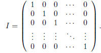
The n· n identity matrix I is the (square) matrix all of whose entries are zero except for those along the
\main diagonal" which are all equal to 1. Symbolically

The   and identity matrices are then

respectively.

The following theorem gives the main ·properties of matrix multiplication. These all follow directly
from the definitions, but some are harder to prove than others, most notably that matrix multiplication is
associative.

Theorem 2. Let A be m· n, B and C be n ·p, D be p· q, and let c be a real number. Then

1. A(B + C) = AB + AC,

2. (B + C)D = BD + CD,

3. (AB)D = A(BD),

4. if I is the m m identity matrix then IA = A,

5. if I is the n· n identity matrix then AI = A,

6. c(AB) = (cA)B = A(cB).

4 Exercises

In exercises 1 and 2, let

and compute each matrix sum or product if it is defined. If it is not defined, explain why.

Exercise 1.

a. A - B

b. A - 3E

c. 2A + DB

d. AC

Exercise 2.

a. A + CB

b. 3BC - A

c. CAD

d. CA - E

Exercise 3. If show that AB ≠ BA but that
AC = CA.
Exercise 4. If construct a nonzero   matrix B (with two distinct columns) so that
AB is the zero matrix.

Exercise 5. If A is an· n n matrix, we say the n· n matrix B is the inverse of A if AB = BA = I,
where I is the n· n identity matrix. Show that if with then the inverse of A is


.
Exercise 6. If and , use the inverse of A (see the previous exercise ) to solve
the matrix equation Ax = b for x.

Exercise 7. If find a nonzero vector v so that Av = 0.