Compound
Interest
Section 4.7
Simple Interest
•Simple Interest Formula
•Principal of P dollars borrowed for t
years at per annum interest rate r
•Interest is I= Prt
•r must be expressed as decimal
Compound Interest
•Payment period
•Annually: Once per year
•Semiannually: Twice per year
•Quarterly: Four times per year
•Monthly: 12 times per year
•Daily: 365 times per year
•Theorem. [Compound Interest
Formula]
The amount A after t years due to a
principal P invested at an annual
interest rate r compounded n times
per year is

•Example. Find the amount that
results from the investment of $1000
at 8% after a period of 8 years.
(a) Problem: Compounded annually
Answer:
(b) Problem: Compounded quarterly
Answer:
(c) Problem: Compounded daily
Answer:
•Theorem. [Continuous Compounding]
The amount A after t years due to a
principal P invested at an annual
interest rate r compounded
continuously is

•Example. Find the amount that
results from the investment of $1000
at 8% after a period of 8 years.
Problem: Compounded continuously
Answer:
Effective Rates of Interest
•Effective Rate of Interest:
Equivalent annual simple interest rate
that yields same amount as
compounding after 1 year.
•Example. Find the effective rate of
interest on an investment at 8%
(a) Problem: Compounded monthly
Answer:
(a) Problem: Compounded daily
Answer:
(a) Problem: Compounded continuously
Answer:
Present Value
•Present value: amount needed to
invest now to receive A dollars at a
specified future time.
•Theorem. [Present Value Formulas ]
The present value P of A dollars to
be received after t years, assuming a
per annum interest rate r
compounded n times per year, is

if the interest is compounded
continuously, then

•Example.
Problem: Find the present value of $5600
after 4 years at 10% compounded
semiannually. Round to the nearest cent.
Answer:
Time to Double an Investment
•Example.
Problem: What annual rate of interest is
required to double an investment in 8
years?
Answer:
Key Points
•Simple Interest
•Compound Interest
•Effective Rates of Interest
•Present Value
•Time to Double an Investment
Exponential Growth and
Decay;
Newton’s Law;
Logistic Growth and
Decay
Section 4.8
Uninhibited Growth and Decay
•Uninhibited Growth:
•No restriction to growth
•Examples
• Cell division (early in process)
•Compound Interest
•Uninhibited Decay
•Examples
•Radioactive decay
•Compute half-life
•Uninhibited Growth:

•N0: initial population
•k: positive constant
•t: time
•Uninhibited Decay

•N0: initial amount
•k: negative constant
•t: time
•Example.
Problem: The size P of a small herbivore
population at time t (in years) obeys the
function  if they have
enough food and the predator population
stays constant. After how many years
will the population reach 1800?
Answer:
•Example.
Problem: The half-life of carbon 14 is 5600
years. A fossilized leaf contains 12% of
its normal amount of carbon 14. How
old is the fossil (to the nearest year)?
Answer:
Newton’s Law of Cooling
•Temperature of a heated object decreases
exponentially toward temperature of
surrounding medium
•Newton’s Law of Cooling
The temperature u of a heated object at a
given time t can be modeled by

where T is the constant temperature of the
surrounding medium, u0 is the initial
temperature of the heated object, and k is
a negative constant.
•Example.
Problem: The temperature of a dead body
that has been cooling in a room set at
70°F is measured as 88°F. One hour
later, the body temperature is 87.5°F.
How long (to the nearest hour) before
the first measurement was the time of
death, assuming that body temperature
at the time of death was 98.6°F?
Answer:
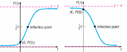
Logistic Model
•Uninhibited growth is limited in
actuality
•Growth starts off like exponential ,
then levels off
•This is logistic growth
•Population approaches carrying
capacity
•Logistic Model
In a logistic growth model, the
population P after time t obeys the
equation

where a, band care constants with
c > 0 (c is the carrying capacity).
The model is a growth model if b >0;
the model is a decay model if b <0.

• Properties of Logistic Function
•Domain is set of all real numbers
•Range is interval (0, c)
•Intercepts:
•no x-intercept
•y- intercept is P (0).
•Increasing if b >0, decreasing if b <0
•Inflection point s when P(t) = 0.5c
• Graph is smooth and continuous
•Example. The logistic growth model

represents the population of a species
introduced into a new territory after t years.
(a) Problem: What was the initial population
introduced ?
Answer :
(b) Problem: When will the population reach 80?
Answer:
(c) Problem: What is the carrying capacity?
Answer:
Key Points
•Uninhibited Growth and Decay
•Newton’s Law of Cooling
•Logistic Model
Building Exponential,
Logarithmic, and
Logistic Models from
Data
Section 4.9
Fitting an Exponential
Function to Data
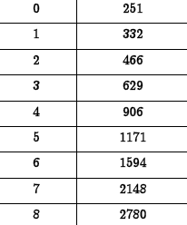
•Example. The
population (in
hundred
thousands) for the
Colonial US in ten-
year increments for
the years 1700-1780
is given in the
following table.
(Source: 1998
Information Please
Almanac)
| Decade, x |
Population, P |
 |
(a) Problem: State whether the data can
be more accurately modeled using an
exponential or logarithmic function.
Answer:
(b) Problem: Find a model for population
(in hundred thousands) as a function of
decades since 1700.
Answer:
Fitting a Logarithmic Function to
Data
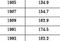
• Example. The
death rate (in
deaths per 100,000
population) for 20-
24 year olds in the
US between 1985-
1993 are given in
the following table.
(Source: NCHS
Data Warehouse)
| Year |
Rate of Death, r |
 |
(a) Problem: Find a model for death rate
in terms of x , where x denotes the
number of years since 1980.
Answer:
(b) Problem: Predict the year in which the
death rate first exceeded 200.
Answer:
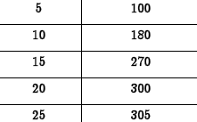
•Example. A
mechanic is testing
the cooling system
of a boat engine.
He measures the
engine’s
temperature over
time.
Time t
(min.) |
Temperature
(°F) |
 |
(a) Problem: Find a model for the
temperature Tin terms of t, time in
minutes.
Answer:
(b) Problem: What does the model imply
will happen to the temperature as time
passes?
Answer:
Key Points
•Fitting an Exponential Function to
Data
•Fitting a Logarithmic Function to
Data
•Fitting a Logistic Function to Data


