Parameterized Timing Analysis

ABSTRACT

Many recent techniques for timing analysis under variability, in
which delay is an explicit function of underlying parameters, may
be described as parameterized timing analysis. The“max” operator,
used repeatedly during block-based timing analysis, causes
several complications during parameterized timing analysis. We
introduce bounds on, and an approximation to, the max operator
which allow us to develop an accurate, general, and efficient
approach to parameterized timing, which can handle either
uncertain or random variations. Applied to random variations,
the approach is competitive with existing statistical static timing
analysis (SSTA) techniques, in that it allows for nonlinear delay
models and arbitrary distributions. Applied to uncertain variations,
the method is competitive with existing multi-corner STA
techniques, in that it more reliably reproduces overall circuit sensitivity
to variations. Crucially, this technique can also be applied
to the mixed case where both random and uncertain variations
are considered. Our results show that, on average, circuit delay is
predicted with less than 2% error for multi-corner analysis, and
less than 1% error for SSTA.

1. INTRODUCTION

Process and environmental variations greatly impact circuit delay,
and can cause parametric yield loss. With the traditional approaches
to timing verification becoming too expensive and unable
to handle local variations, new alternatives have emerged in
recent years, most of which can be described under the heading
of parameterized timing analysis. Essentially, timing quantities
are “parameterized” as explicit functions of the underlying process
and environmental parameters, allowing one to assess the
effect of these parameters on circuit delay, which can be useful
in determining the robustness of the design and its sensitivity
to variations. It is worth mentioning that process variations1,
which are manufacturing variations or mismatches between transistor
parameters, are statistical variations and can be modeled
as random variables (RVs), while environmental variations, which
are operating context variations, are non-random and must be
treated as uncertain parameters. Both types of variations must
be taken care of in the context of parameterized timing analysis.
 

One of the major trends in parameterized timing analysis is
block-based statistical static timing analysis (SSTA) [1, 7, 2, 8,
9, 4, 6, 3], where parameters are modeled as RVs. In the past
few years, several SSTA techniques have been proposed. In [1,
7], linear-time techniques were proposed using linear (first-order)
delay models and Gaussian distributions for process parameters,
which allows the use of tightness probability to resolve the max
operation efficiently. It is expected, however, that nonlinearities
will increase with technology scaling. On one hand, as the magnitude
of process variations is increasing, first-order delay models
are no longer accurate. Also, there is evidence that delay is
highly nonlinear in low-voltage modes. On the other hand, process
variations are not necessarily Gaussian. For example gate
length has an asymmetric non-Gaussian distribution due to variation
in depth of focus (DOF). To address these concerns, several
attempts were made to generalize SSTA in order to handle nonlinear
delay models and/or random variables with non -Gaussian
distributions. In [8, 9], despite the use of quadratic models, Gaussian
distributions were forced on process parameters. In [6], non-
Gaussian process parameters were addressed, but first-order linear
models were used. Recently, both non-Gaussian parameters
and nonlinear models were addressed simultaneously, with varying
degrees of success. In [4], a sampling (Monte Carlo) based
regression is used to handle the max operation, which increases
the overall runtime; [2] uses expensive multi-dimensional integration
to handle the nonlinear non-Gaussian terms, which hinders
the complexity of the approach; [3] proposes an efficient nonlinear
non-Gaussian SSTA technique with linear complexity. This technique
uses Fourier series and moment matching to approximate
the max operation efficiently. The drawback of this approach is
that it requires subdividing the region of variation of every variation
source, then for every sub-region, the Fourier transform of
every possible distribution used is pre-computed. Although this is
done as a pre-processing step, it can introduce undesired complications,
especially if these distributions are unknown . In addition,
by using moment matching and being distribution dependent, all
these SSTA techniques fail to handle uncertain non-random parameters,
which is a requirement in general parameterized timing.

Another type of parameterized timing analysis is linear-time
multi-corner static timing analysis (STA), which was introduced
in [5]. The idea is to propagate hyperplanes, i.e., affine linear
functions of the process and environmental parameters, in the
timing graph. The max operation is resolved by raising the hyperplanes
in a way to always follow the maximum corner delay.
In this way, the circuit maximum corner delay is estimated accurately.
Although the approach can handle both random and
uncertain parameters, it has some drawbacks: while trying to be
always accurate at the maximum corner delay, the approach loses
accuracy at the other corners. Consequently, the sensitivity to
process variations is lost and this approach can not be used for
optimization because the true spread of the circuit delay is not
accurately estimated. In addition, the analysis is restricted to
linear delay models.

In this work, we propose an efficient and general parameterized
timing analysis technique that can handle nonlinear delay models
and account for delay variability due to both random process
parameters with arbitrary (and possibly unknown) distributions
and uncertain non-random parameters (that typically may depend
on the operating environment). Our technique is based on
a novel and efficient method to resolve the nonlinear max operator
by either bounding or approximating it by a linear model,
while preserving the inherent nonlinearity of the delay model itself.
We have tested our technique within two timing verification
frameworks, namely multi-corner timing analysis and nonlinear
non-Gaussian SSTA, and have shown that, at least when using
quadratic delay models, the complexity of the approach is linear
in both the number of process and environmental parameters and
the circuit size. Our results show that the spread of the maximum
circuit delay is accurately captured, whereby, on average,
the maximum and minimum corner delays are predicted with less
than 2% error for multi-corner analysis. As for nonlinear non-
Gaussian SSTA, all timing characteristics are predicted with less
than 1% average error.

2. GENERAL PARAMETERIZED TIMING

In general, the delay of gates and interconnects is a nonlinear
function that can be approximated using a delay model that
depends on the underlying process and environmental variations.
As stated earlier, linear (first-order) and quadratic (second-order)
delay models have been previously used in the literature. Nevertheless,
for the time being, we will work under the assumption of
an arbitrary delay model; we will show later that our approach
can be used with a general class of nonlinear delay models. We
can write the delay D of gates or interconnects as follows:

where f_D(·) is an arbitrary delay model, and X_i’s represent process
and environmental variations. Recall that not all variations
can be modeled as random variables. While some parameters are
indeed random such as channel length or threshold voltage, others
are not statistical but rather uncertain parameters, such as temperature
or supply voltage. These parameters typically depend
on the operating environment. We will show that our analysis is
indifferent to whether parameters are random or uncertain and
thus the approach can be applied for both types of variations.

The benefit of parameterized timing analysis is in elevating the
explicit delay dependence on process and environmental variations,
i.e., the delay model, from the stage level to the circuit
level, allowing one to assess the effect of these parameters on the
total circuit delay. In block-based timing analysis, this is done by
propagating timing quantities in the timing graph in topological
order, using a sequence of basic operations, such as add operations
on arrival times and arc delays, and max operations on the
timing quantities resulting from those additions in order to get
the output arrival time. If these basic operations do not distort
the delay model at hand, then circuit delay can be represented in
the same delay model. Unfortunately, it is known that the max is
nonlinear. The novelty of this work is in resolving the nonlinear
max operator using a linear model, while preserving the inherent
nonlinearity of the delay model.

In the following section, we propose two methods to efficiently
resolve the max: first by using upper and lower bounds , and
second by using an approximation that minimizes the square of
the error . Our methods operate irrespective of the delay model
used provided it falls in a general class of nonlinear functions;
they also handle random parameters with arbitrary distributions,
as well as uncertain parameters. In the rest of the paper, we
will refer to random and uncertain parameters simply as process /
environmental parameters.

3. MATHEMATICAL FRAMEWORK

3. MATHEMATICAL FRAMEWORK
Let F be a general class of (possibly) nonlinear functions that
obey the following three properties,

1. F is closed under linear (and/or affine) operations

is bounded

can be maximized and minimized efficiently
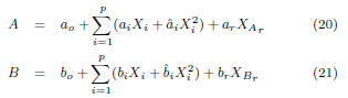
and assume that all timing quantities are represented using delay
models that are in F. For example, timing quantity A is modeled
as follows:

where X = [X₁, · · · ,X_p] represent process/environmental parameters.

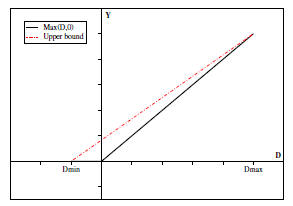
Figure 1: Upper bound on Y

The first property essentially states that linear operations (such
as addition or subtraction) will result in functions that belong
to F; in other words, F “survives” linear operations, that is, if
A = f_A(X) ∈ F and B = f_B(X) ∈ F, then C = aA + bB + c,
where [a, b, c] ∈ R, will be such that C = f_C(X) ∈ F. Note
that all polynomial models satisfy this property. The second and
third properties imply that the delay model, and consequently
any timing quantity expressed using the model, is bounded by a
minimum and a maximum value over the space of parameters, i.e,
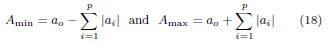
A_min ≤ A ≤ A_max, where:

Note that the second property is trivial if we recall that all physical
process and environmental parameters are bounded, which
implies that delays are also bounded. The third property is only
forced to guarantee that our approach, which requires maximizing
and minimizing the delay model in order to operate, is computationally
efficient. For instance, if maximizing/minimizing the
delay model is linear (in the process/environmental parameters),
then the overall complexity of our approach is linear in the circuit
size and process/environmental parameters. By property 1,
it is clear that the add operation, being linear, will maintain their
membership in F as delay models are propagated during timing
analysis. However, the max operation, being nonlinear in general,
is the crux of the problem, and we now focus on it.

3.1 Max Operation

Let A and B be two timing quantities expressed using delay
models in F. Let C = max(A,B) be the maximum of A and
B. Since the maximum operator is, in general, nonlinear, then C
is not necessarily expressible using a delay model in F. We are
interested however in finding (1) two bounds on C, C_l and C_u,
and (2) an approximation C_a, which can all be expressed using
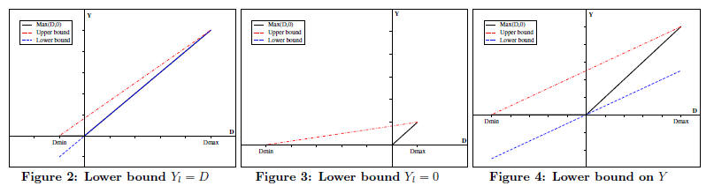
functions in F, and such that:

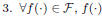
where D = A − B and Y = max(D, 0).

Recall from property 1 that F survives linear operations (including
subtraction), which means that D = f_D(X) ∈ F. By
properties 2 and 3, D is bounded and varies between [D_min,D_max]
where D_min ≤ D_max. Depending on the signs of these extreme
values of D, we can identify two cases in which the max operator
is either linear or nonlinear. If D_min ≥ 0 then , and
Y = D. In this case, C = A since A completely dominates B.
The converse happens when D_max ≤ 0; in this case, C = B, since
B completely dominates A. The more interesting case is when
the max is nonlinear, which can be identified when D_max ≥ 0
and D_min ≤ 0. In this case, which we will refer to by saying that
A and B are co-dominant, Y = max(D, 0) can not be expressed
using a delay model from F. We will now show how we can bound
and approximate Y using functions that belong to F.

3.2 Bounding the Max

3.2.1 Upper bound
Fig. 1 shows a broken solid line representing a plot of Y =
max(D, 0) between D_min and D_max, the extreme values of D. We
are interested in finding a linear function of D that is guaranteed
to upper bound Y (recall, since D ∈ F, then any linear function
of D is also a member of F). The dashed line represents an affine
function of D which upper bounds Y and is exact at D_max and
D_min. Note that the bound is closer to the exact max around
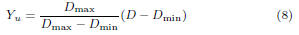
D_min and D_max where either A or B dominates. The equation
for Y_u, the upper bound on Y , can be expressed as follows:

By replacing Y with Y_u in (7), we get an upper bound C_u on C:

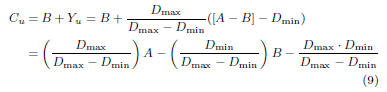
Note that 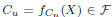since it is a linear combination of
A and B (property 1). To gain a more intuitive understanding of
the above relationship, let us define the following terms:

• S = D_max − D_min to be the “spread” of D
• S_A = D_max to be the “strength” of A, i.e. the region where A dominates B (D ≥ 0)
• S_B = −D_min = |D_min| to be the “strength” of B, i.e. the region where B dominates A (D ≤ 0)
• α = S_A/S is the fraction of space where A dominates B
• (1 − α) = 1 − S_A/S = S_B/S is the fraction of space where B dominates A

Then, using the above notations, we can rewrite C_u as follows:

where A and B are both weighted by their “extent of dominance”,
so to speak, and the last term accounts for the region where both
A and B are dominant, hence the product of α and (1 − α).

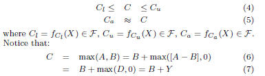
3.2.2 Lower bound

Similarly, we would like to find a lower bound on Y in order to
find a lower bound C = max(A,B). Looking back at Fig. 1, it is
easy to see that any function in the form Y_l = aD, where 0 ≤ a ≤
1, is a valid lower bound on Y = max(D, 0) and can be expressed
using a function in F (property 1). In practice, we have found
that limiting the choice of Y_l to one of three functions depending
on the values of D_min and D_max is sufficient. Figures 2-4 depict
these three cases. In addition to showing Y in solid line and upper
bound Y_u in dashed line, these figures show the lower bound Y_l
to be one of the following:

where the slope of Y _l in the third case is equal to that of the
upper bound Y_u. Note that means “much larger than”, and it
was set to be at least 4 times larger in our simulations.
Replacing each case of the above in (7) gives us C_l, the lower
bound on C:

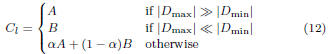
where α is as defined in (10). Therefore, since
it is a linear combination of A and B (property 1).

3.3 Least Squares Max Approximation

In the previous sections, we have shown how we can determine
upper and lower bounds on C = max(A,B) using a carefully
chosen linear combination of A and B. We are now interested
in finding an expression C_a that approximates C = max(A,B)
and can be expressed using a function that belongs to F. To do
that, it suffices to approximate Y = max(D, 0) in (7) by a linear
approximation Y_a in the form Y_a = aD + b. We will choose a
and b in such a way to minimize the sum of the squares of the
error inside the interval [D_min,D_max]; we call this approximation
the least squares max approximation. It is understood that this
approximation is applied only when the max is nonlinear, i.e., in
the case of co-dominance.

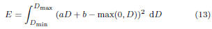
Let E be the total error incurred by the above approximation.
Then we can express E as follows:

We now determine the parameters a and b that minimize E.
To do that, we first determine the partial derivatives of E, ∂E/∂a
and ∂E/∂b , with respect to a and b, then we set the derivatives to
zero and solve for a in b. This gives us the following two equations
in a and b:

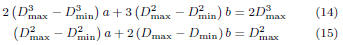
Finally, a and b can be easily obtained by solving the system of
equations (14) and (15), which result in:

C_a can be easily obtained by replacing Y with Y_a = aD + b
in (7). It is easy to see that 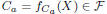since it is a linear
combination of A and B which are in F (property 1). Fig. 5

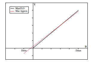
Figure 5: Least squares Max approximation

shows the true max, Y = max(D, 0) in solid line, and the least
squares max approximation, Y_a = aD + b, in dashed line.

To summarize, we have presented a mathematical framework
that resolves the nonlinear max operator in two ways; either by
using bounds, or by using an approximation that minimizes the
error with the true max. This framework is simple and general,
in the sense that it can be applied to a general class of nonlinear
delay models, and it uses simple linear operations, allowing
to keep and propagate the same delay model to later stages. In
addition, the analysis is indifferent (1) to whether the variation
sources are modeled as random variables or uncertain variables,
or (2) to the types of distributions used, when the variations are
random. In spite of its apparent simplicity, we will now demonstrate
that this approach is extremely effective and competitive in
dealing with two difficult application areas: multi-corner timing
analysis as well as nonlinear non-Gaussian SSTA. Crucially, this
approach can also deal with the “mixed” case, which is typical
of practical situations, where some variables are random while
others are simply uncertain.

4. MULTI-CORNER STA

In corner case analysis, circuit timing must be checked at various
process/environmental corners, which are typically extreme
values of process/environmental parameters. This approach to
timing verification is exponential in the number of varying parameters
as multiple runs of STA are needed to cover all possible
corners in order to determine the maximum and minimum
corner delays. Instead, in practice, using parameterized timing,
where timing quantities are expressed using a variational delay
model that depends on process and environmental parameters,
one hopes to do this task with only one traversal of the timing
graph; this is what we call linear-time multi-corner STA.

In this section, we demonstrate how our simple framework can
handle this otherwise complex analysis in a simple and elegant
fashion. To our knowledge, and unlike [5], where the approach
is restricted to linear delay models, we are the first to handle,
in linear-time, multi-corner STA with linear and nonlinear delay
models alike. In order for our framework to hold, all we need
to show is that the three properties of section 3 are satisfied.
For illustration, we will demonstrate our approach for linear and
quadratic models.

4.1 Linear and Nonlinear Models

Let F₁ and F₂ be the sets of linear and quadratic delay models
respectively. Let A be a timing quantity such that:

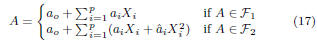
where a_o is the nominal delay of A, and a_i and are first-order
and second-order sensitivities to X_i. Note that X_i’s are arbitrary
variation sources (random/uncertain variables) that are bounded,
and without loss of generality, assume that −1 ≤ X_i ≤ 1.

It can be easily shown that property 1 holds, i.e., both F₁ and
F₂ survive linear operations. In fact, if [A,B] ∈ F₁, then C =
aA+bB +c also ∈ F₁. The same applies for F₂. Property 2 also
holds, since X_i’s are bounded. As for property 3, both the linear

and the quadratic model can be easily maximized and minimized
in O(p) time, where p is the number of process/environmental
parameters; if A ∈ F₁, then:

whereas, if A ∈ F₂, then maximizing and minimizing A over the
space of variations requires maximizing and minimizing the individual
quadratic terms, 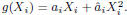In the Appendix,
we show how this can be done analytically depending on whether
g(X_i) is monotone in [−1, 1] or not. Therefore maximizing and
minimization A is linear in the number of parameters, since there
are p quadratic terms.

Given that all the required properties are satisfied by F₁ and
F₂, the methods described in sections 3.2 and 3.3 for resolving
the max operation can be applied to demonstrate multi-corner
STA with linear and nonlinear delay models. The timing graph is
traversed topologically, and our bounding/approximation scheme
is applied to handle the max operation at every stage. This results
in expressing the arrival time at the sink node, i.e., the maximum
circuit delay, using the delay model at hand. Once this expression
is obtained, it can be easily maximized and minimized as shown in
this section to bound/approximate the maximum and minimum
corner delays of the maximum circuit delay.

4.2 Results

We have tested our approach by first characterizing a 90nm
CMOS library using HSPICE in order to determine the sensitivities
of gate delay to various process parameters. We have chosen
to vary channel length (L_n and L_p), and threshold voltage (V_tn
and V_tp) of NMOS and PMOS transistors, and have determined
the sensitivities of gate delays to these process parameters. The
variation information was specified in the technology files. Our
technique was then implemented using C/C++ and was tested on
the ISCAS85 benchmark circuits. For each circuit, the maximum
circuit delay is determined at various corners using exhaustive
corner case analysis, and the true maximum and minimum corner
delays are recorded. Our framework is then applied, using (1)
the lower bound technique, (2) the upper bound technique, and
(3) the least squares approximation, to predict the maximum and
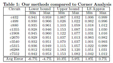
minimum corner delay for every circuit. The results are summarized
in Table 1, where the values shown are normalized to the
true minimum and maximum corner delays respectively, determined
by corner case analysis. For example, the second column
gives a lower bound on the minimum (over all corners) circuit delay,
and the last column gives an approximation of the maximum
(over all corners) circuit delay. The closer the values are to 1 the
more accurate they are. Note that, unlike [5] where the method
is only accurate in predicting the circuit delay at the maximum
corner, we can accurately estimate the maximum circuit delay at
both the minimum and the maximum corners, so that the spread
of the maximum circuit delay is well-captured. In addition, our
approach is not restricted to linear models. The last row of the
table shows the average percent error for every approach; the
maximum and minimum corner delays can be approximated up
to 0.7% and 1.8% respectively.

5. NONLINEAR NON-GAUSSIAN SSTA

We now demonstrate nonlinear non-Gaussian SSTA, using a
general quadratic delay model that depends on process variables
modeled as RVs with arbitrary distributions, as well as uncertain
non-random parameters. As has become typical in the SSTA
literature [1], we assume that one can deal with within-die correlations
using some simple scheme by which correlation is resolved
based on the physical location of a cell on the layout surface. As a
result, when it comes to those variations which are random variables
(as opposed to the uncertain non-random parameters), we
assume that we are only dealing with global variations and purely
random variations. Before proceeding with the details, we first
show how the three properties of the delay model are satisfied in
order for our framework to hold.

5.1 Delay Model

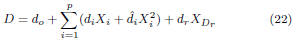
Assume that gate delay D is expressed using a quadratic model,
F, as follows:

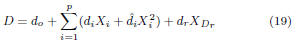
where d_o is the nominal delay, d_i and are first-order and second-order
sensitivities to X_i, and d_r is the sensitivity to the purely
independent random variation specific to D.

Because our framework is indifferent to whether parameters
are random or uncertain, there is no restriction on X_i’s, which
can be either RVs or uncertain non-random parameters alike. If
it is random, X_i is modeled as an independent zero mean RV
with an arbitrary distribution, such that −1 ≤ X_i ≤ 1. This can
be any distribution, including common cases such as a truncated
Gaussian (normal) distribution, a uniform distribution, etc. If it
is uncertain, X_i is simply assumed to vary in [−1, 1]. Note that,
in both case, X_i’s are global variation sources that are shared
by all gate delays and timing quantities. As for the purely independent
random variation , we will assume that it can be
modeled as a standard normal distribution with zero mean and
unit variance. This is because are typically the result of
various independent random effects that add up and converge to
a normal distribution by the central limit theorem.

5.1.1 Add Operation

The add operation and generally any linear operation can be
easily performed without destroying the above quadratic model.
Assume that [A,B] ∈ F:

then C = aA+bB+c can be expressed using the quadratic model
as follows:

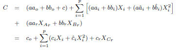
wher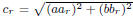e since are independent
standard normal RVs, and is an independent standard
normal RV specific to C. Therefore, F satisfies property 1.

5.1.2 Max Operation

As explained in section 3, the max operation C = max(A,B)
is resolved by first subtracting A and B , i.e., D = A − B and
then bounding/approximating C using linear combinations of A
and B; recall that the coefficients of the linear combinations are
functions of the minimum and maximum values of the difference
D, i.e., D_min and D_max.

We have already shown how to perform linear operations using
the quadratic model. Hence, in order to apply the results of
section 3, it remains to show how the quadratic model is bounded
and can be efficiently maximized and minimized over the space
of variations (properties 2 and 3). Assume that we have already
performed the subtraction D = A − B, and D is given by:

Since X_i’s and are all independent, then the maximum D_max
and minimum D_min of D are achieved when all variations are
maximized and minimized separately. In other words, we need to
maximize and minimize the quadratic terms and the independent
random term.

The quadratic terms 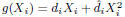can be analytically
maximized and minimized as shown in the Appendix. As for
the purely independent random variation , recall that it is
modeled as an RV with standard normal distribution, which suggests
that can take values in −∞ to +∞. This, however,
is not realistic, and it is usually the case that standard normal
distributions are truncated between [−k, k], where k represents
multiple standard deviations. As an example, setting k = 3 will
cover 99.73% of the standard normal distribution. As a result,
the maximum and minimum values contributed by the independent
random component are kd_r and −kd_r respectively. Hence,
by combining the above two contributions, D_min and D_max can
be easily determined. Having shown that the three properties of
section 3 are satisfied by F, we use the approaches in sections 3.2
and 3.3 to resolve the max operation.

5.2 Complexity Analysis

We have shown that both add and max operations are resolved
using simple linear operations involving the delay model; in addition,
the coefficients of the linear combination needed for the max
operation involve a subtraction and a maximization/minimization
performed on the model. If p is the total number of variation
sources, then performing an addition or a subtraction is O(p);
also, performing a maximization/minimization of the model is
O(p). This means that both add and max operations are linear in
the number of variation sources. Therefore, the overall complexity
of a block-based SSTA technique using the above operations
is O(pn), where n is the circuit size.

5.3 Results

We have implemented our nonlinear non-Gaussian block-based
SSTA technique using C/C++ and have tested it on the ISCAS85
benchmark suite. Similarly to [3], and as a proof of concept, we
have generated the variation information randomly. We have chosen
the coefficients of the quadratic delay model in such a way that
every variation source causes 10% to 20% deviation in the nominal
delay. In addition to the purely random variation which follows a
truncated Gaussian distribution, 4 global variation sources X_i’s
were used, each following either a truncated Gaussian, a uniform,
or a triangular distribution as shown in Fig. 6. The accuracy of
our technique is compared to Monte Carlo analysis with 10, 000
runs. All delays reported are normalized to the nominal circuit
delay. Fig. 7 shows a plot of the cumulative distribution functions
(CDF) for benchmark c1355 for the case of variations with
a uniform distribution, generated using our SSTA technique and
compared to Monte Carlo simulation. Note that the bounds are
valid and accurate, and the least squares (LS) approximation is
very close to the true distribution. Table 2 compares the following
timing metrics: the 95 and the 99 delay percentiles, and the
ratio of standard deviation to the mean σ/μ, generated using the
least squares approximation (LS-SSTA) to Monte Carlo analysis,
for Gaussian, uniform, and triangular distributions. The results
show that our approach is consistently accurate for all metrics
and different distributions, with an average error less than 1%.

In the mixed case, where one is dealing with both random
variables and uncertain variables, the overall (random) circuit
delay and the interesting statistical metrics (like mean, variance,
percentiles) are effectively functions of the uncertain variables. If
this functional dependence is complex, then the desirable worstcase
values (of the interesting statistical metrics) must be found
by a process of search or optimization. This type of follow-up
analysis is beyond the scope of this paper, and is the topic of our
continued work under this project. For now, the above results
were obtained at a specific setting (the nominal) of the uncertain
variables. This does not diminish the value of the results, because
one strength of our existing approach is that it provides an explicit
dependence of the total circuit delay on the uncertain parameters,
so that one does not simply have to repeat the overall SSTA for
different settings.

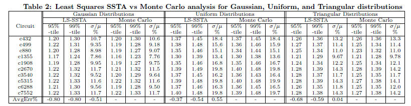
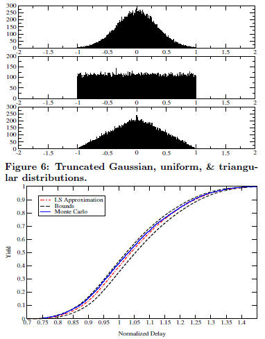
Figure 7: CDF comparison for c1355.

6. CONCLUSION

We have proposed a general parameterized timing analysis technique
that can handle nonlinear delay models and account for delay
variability due to both random process parameters with arbitrary
distributions and uncertain non-random parameters which
depend on the operating environment. Central to this technique
is a novel and efficient method to resolve the max operator by
bounding it and approximating it using linear models, while preserving
the inherent nonlinearity of the delay model itself. We
have tested our technique within two timing verification frameworks,
namely multi-corner timing analysis and nonlinear non-
Gaussian SSTA, and have shown that the complexity of the approach
is linear in both the number of process and environmental
parameters and the size of the circuit. Our results show that,
on average, circuit delay is predicted with less than 2% error for
multi-corner analysis, and less than 1% error for SSTA.

APPENDIX

For completeness, we show the (simple) process by which one can
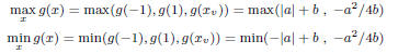
maximize or minimize a quadratic function of the form, g(x) =
ax+bx^2, where −1 ≤ x ≤ 1, and [a, b] ∈ R. Recall that the minimum/
maximum is at x_v = −a/(2b). If x_v falls outside [−1, 1]
then g(x) is monotone in [−1, 1], so that its maximum and minimum
occur at the domain boundaries:

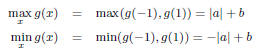
On the other hand, if x_v falls in [−1, 1], then g(x) is not monotone
in [−1, 1], i.e., the maximum and minimum can be either at the
vertex or at the boundaries of the domain: