Definition. A system of m linear equations in the n
unknowns 
is a system of the form :
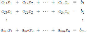
Note. The above system can be written as
 where A is the
coefficient matrix and  is the vector of
variables. A solution to the
system is a vector  such that
 .
.
Definition. The augmented matrix for the above
system is
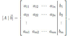
Note. We will perform certain operations on the
augmented matrix which
correspond to the following manipulations of the system of equations:
1. interchange two equations ,
2. multiply an equation by a nonzero constant,
3. replace an equation by the sum of itself and a multiple of another
equation.
Definition. The following are elementary row operations:
1. interchange row i and row j (denoted  ),
),
2. multiplying the ith row by a nonzero scalar s (denoted
 ),
),
and
3. adding the ith row to s times the jth row (denoted
 ).
).
If matrix A can be obtained from matrix B by a series of elementary row
operations, then A is row equivalent to B , denoted A ~B or A → B.
Notice. These operations correspond to the above manipulations of the
equations and so:
Theorem 1.6. Invariance of Solution Sets Under Row
Equivalence.
If  then the linear systems
 and
and
 have the
same solution sets.
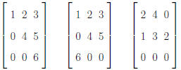
Definition 1.12. A matrix is in row-echelon form if
(1) all rows containing only zeros appear below rows with nonzero entries,
and
(2) the first nonzero entry in any row appears in a column to the right of
the first nonzero entry in any preceeding row .
For such a matrix, the first nonzero entry in a row is the pivot for that
row.
Example. Which of the following is in row echelon form?
Note. If an augmented matrix is in row-echelon
form, we can use the
method of back substituton to find solutions .
Example. Consider the system

Definition 1.13. A linear system having no solution
is inconsistent. If
it has one or more solutions, it is consistent.
Example. Is this system consistent or inconsistent:

Example. Is this system consistent or inconsistent:

(HINT: This system has multiple solutions. Express the
solutions in terms
of an unknown parameter r).
Note. In the above example, r is a “free variable”
and the general
solution is in terms of this free variable.
Note. Reducing a Matrix to Row-Echelon Form.
(1) If the first column is all zeros, “mentally cross it off.” Repeat this
process as necessary.
(2a) Use row interchange if necessary to get a nonzero entry (pivot) p in
the top row of the remaining matrix.
(2b) For each row R below the row containing this entry p, add −r/p
times the row containing p to R where r is the entry of row R in the
column which contains pivot p. (This gives all zero entries below pivot p.)
(3) “Mentally cross off” the first row and first column to create a smaller
matrix. Repeat the process (1) - (3) until either no rows or no columns
remain.
Example. Page 68 number 2.
Example. Page 69 number 16. (Put the associated augmented matrix
in row-echelon form and then use substitution.)
Note. The above method is called Gauss reduction
with back substitution.
Note. The system
 is equivalent to the
system

where  is the ith
column matrix of A. Therefore,
 is consistent
if and only if  is in the span of
 (the columns of A).
Definition. A matrix is in reduced row-echelon form
if all the pivots
are 1 and all entries above or below pivots are 0.
Example. Page 69 number 16 (again).
Note. The above method is the Gauss-Jordan method.
Theorem 1.7. Solutions of
 .
.
Let
 be a linear system and let
  where H is in
row-echelon form.
(1) The system
 is inconsistent if and only if
 has a row
with all entries equal to 0 to the left of the partition and a nonzero entry
to the right of the partition.
(2) If  is consistent
and every column of H contains a pivot, the
system has a unique solution.
(3) If  is consistent
and some column of H has no pivot, the
system has infinitely many solutions, with as many free variables as there
are pivot-free columns of H.
Definition 1.14. A matrix that can be obtained from an identity matrix
by means of one elementary row operation is an elementary matrix.
Theorem 1.8. Let A be an m × n matrix and let E be an m × m
elementary matrix. Multiplication of A on the left by E effects the
same elementary row operation on A that was performed on the identity
matrix to obtain E.
Proof for Row-Interchange. (This is page 71 number 52.) Suppose
E results from interchanging rows i and j:

Then the kth row of E is [0, 0, . . . , 0, 1, 0, . . . ,
0] where
(1) for  the nonzero
entry if the kth entry,
(2) for k = i the nonzero entry is the jth entry, and
(3) for k = j the nonzero entry is the ith entry.
Let  , and
, and  .
The kth row of B is
 and
and

Now if  then all
 are 0 except for p = k and

Therefore for  , the kth
row of B is the same as the kth row of
A. If k = i then all  are 0 except for p = j
and

and the ith row of B is the same as the jth row of A.
Similarly, if k = j
then all  are 0 except for p = i and

and the jth row of B is the same as the ith row of A.
Therefore

Example. Multiply some 3 × 3 matrix A by
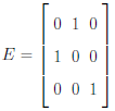
to swap Row 1 and Row 2.
Note. If A is row equivalent to B, then we can find C such that CA = B
and C is a product of elementary matrices.
Example. Page 70 number 44.


