Introduction to Matrix Operations

Introduction to Matrix Operations
Matrices, the representation of a set of numbers in a uniform array, are used widely in
engineering applications. From high end computer analysis packages to simple data
bases, a matrix is a compact and useful tool in engineering analysis.

In this handout, we briefly cover the rules of fundamental matrix operations and a few
examples of how they are used for solving systems of equations .

Matrix representation

A matrix can be a large array of numbers denoted by a single symbol. The symbol used to
represent the matrix is usually in bold font, or alternately, underlined.

For example:

R is called a 2 x 3 matrix (2 rows by 3 columns). In Matlab, we would enter the matrix
into the workspace using the following command.
>> R = [3 8 10;-4 6 5];

We can refer to a single element of the matrix by specifying the elements position in the
matrix, it's row and column number. For example, in R, the 2,3 element (2^nd row, 3^rd
column) is 5.

n Matlab, we place the row and column numbers in parentheses . These numbers are
called indices into the matrix.

>> R(2,3)

would return the 2,3 element, which is 5.

Matrix Addition and Subtraction .

Addition and subtraction of matrices is straightforward. The sum of two matrix is the
result of summing the element individually. AN important implication of this definition
is that the two elements being summed must be of the same dimensions (same numbers
of rows and columns.

Let:

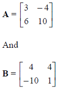
Then, if C = A + B,

Matrix Multiplication

Multiplication of two matrices is more complicated. Essentially the rows of the first
matrix are combined with the columns of the second matrix in a systematic fashion. The
expression below shows the general rule.

where

Dimensional consistency is an important aspect of matrix multiplication. The above rule
implies that the number of columns in the first matrix must be equal to the number of
rows in the second matrix. The resulting matrix has the same number of rows as the first
and the same number of columns as the second. When MATLAB generates and error
message that "inner dimensions must agree" it has found a case in which you are
attempting to violate this rule.

Systems of equations and matrix multiplication

To get a better understanding of these issues, consider the following two problems, one
taken from sophomore mechanical and civil engineering classes (ENGR 210) and one
taken from sophomore electrical engineering classes (ENGR 240).

Problem 1: Equilibrium Mechanics.

The figure below shows a pickup truck undergoing acceleration. We know the mass of
the pickup truck, the location of the center of gravity and the magnitude of the
acceleration. Find the force experienced at the tires (R₁, R₂, and R₃).

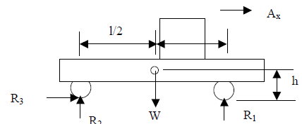
From the principles of equilibrium and Newton second law of motion , we can write the
following three equations involving the unknown forces on the tires:


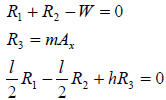
The mass of the pickup is approximately 1000 kg and it is accelerating at 3 m/s/s. The
physical dimensions l and h are also known, l = 3 m and h = 0.5 m. The above three
equations make up a system of three equations and three unknowns. These can be placed
in matrix form and we can let Matlab help up solve them.

First, we must put the equations in matrix form. Start by realizing that all three equations
can be seen to involve all three unknowns, just some of them have coefficients of zero .


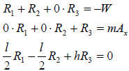
Keeping in mind the definition of matrix multiplication, we can put this system in matrix
form:

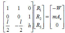
If we use symbols to represent the three matrices, you can represent this equation as
shown below:

A R = B

We solve this equation (that is, find values for the forces in R), by the process of matrix
inversion. The inverse of a given matrix is that matrix, which will yield the identity
matrix when multiplied by the original matrix. Keeping with the above equation, we can
multiply both sides by the identity matrix:

A^-1 A R = A^-1 B

Which simplifies to:

R = A^-1 B

Matlab makes this easy. Given the values that were give for this problem, we can easily
enter the matrices:

>> A=[1 1 0;0 0 1;1.5 ?.5 0.5]
>> B=[1000*9.81;1000*3;0]
>> R= inv(A)*B

It is left to the student to compute the final answers and verify their correctness.

Problem 2: Multiple Loop Circuits

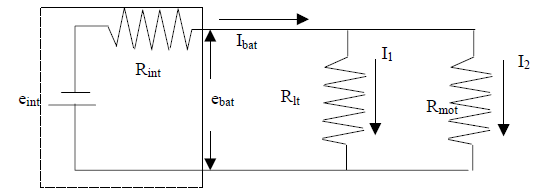
The sketch below shows a circuit that can be used to model a battery powering two loads
in parallel, say a motor and a light bulb. The chemical reaction inside the battery provides
an electrical potential of about 1.5 volts but internal losses make the actual voltage on the
battery terminals somewhat less. These losses are modeled by an internal resistance.

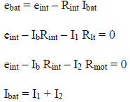
Using basic principles of circuit analysis, we can easily right the following 4 equations
summarizing the circuit behavior.



It is left to the student to verify that the matrix form below is a proper representation of
the previous 4 equations.


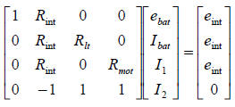
If R_int = 5 ohms, R_1t= 100 ohms, R_mot = 50 ohms and e_int = 1.5 volts, solve this problem.