COMPUTER PROJECT FOR MATH2605

1. Project Preparations

1) Implement Gaussian elimination. Suggestion:
void gaussianElimination(Matrix_nxn *A, Vector_n *b,
Vector_n *sol);

(2) Implement Gaussian elimination with partial pivoting. Suggestion:
void gaussianEliminationPivoting(Matrix_nxn *A, Vector_n *b,
Vector_n *sol);

(3) Implement the QR decomposition using Gram-Schmidt. Suggestion:
void QR_gramSchmidt(Matrix_nxn *A,
Matrix_nxn *Q, Matrix_nxn *R);

(4) Implement the QR decomposition using Householder reflections. Suggestion:
void QR_householder(Matrix_nxn *A,
Matrix_nxn *Q, Matrix_nxn *R);

5) Implement solving a linear equation using QR decomposition. Suggestion:
void solve_QR(Matrix_nxn *Q, Matrix_nxn *R, Vector_n *b,
Vector_n *sol);

(6) Implement solving a linear equation using Gauss-Seidel iteration. Suggestion:
void solve_GaussSeidel(Matrix_nxn *A, Vector_n *b,
double precision,
Vector_n *sol);

(7) Implement solving a linear equation using Jacobi iteration. Suggestion:
void solve_Jacobi(Matrix_nxn *A, Vector_n *b,
double precision,
Vector_n *sol);

You are free to use any programming language of your choice to implement the
algorithms. You are allowed to use basic vector, matrix operations ( addition , multiplication,
dot- products and norms ) provided by libraries and/or the programming language.

As far as notation of the project description is concerned, let

for any n-vector v and any n × n matrix A.

As a criterion to stop the iteration algorithms I would suggest you to choose
either one of the following after computing x_n+1 out of x_n

then stop. (The latter case is
counted as if the algorithm did not converge.)

then stop. (The latter case is counted
as if the algorithm did not converge.)

where ε is the relative error tolerance (e.g. ) and N the maximum number
of iteration steps your are willing to spend (e.g. ).

The requested plots can be generated by whichever software you can use. It is
definitely not asked to write software for that part of the project.

2. Project – Part 1

For any matrix size n≥2 consider the n × n matrix

For matrix sizes

n = 3, 4, 5, . . . , 20

do

• Compute the QR decomposition of A using Gram-Schmidt and Householder.
• Check the quality of your result of Q by computing

for both decompositions.

• Check the quality of your result of Q and R by computing

for both decompositions.

Summarize your finding by plotting against n
for both methods . Try to explain your results (a few sentences are enough).

3. Project – Part 2

For any matrix size n≥2 let A be the matrix of equation (1), and let the vector
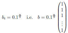
b be given by

For matrix sizes

n = 3, 4, 5, . . . 20

try to find the solution to Ax = b by using

(1) Gaussian elimination.
(2) Gaussian elimination with partial pivoting.
(3) Computing first a Q-R decomposition of A using Gram-Schmidt, and solving
Rx = Q^Tb using only the back-substitution part of the Gaussian
elimination algorithm.
(4) Computing first a Q-R decomposition of A using Householder, and solving
Rx = Q^Tb using only the back-substitution part of the Gaussian elimination algorithm.
(5) Using Jacobi iteration (e.g. start with x₀ = 0)
(6) Using Gauss-Seidel iteration (e.g. start with x₀ = 0)

Summarize your findings by plotting against n for all the above
algorithms. Try to explain your result (in a few sentences).

4. Project – Part 3

For any matrix size n≥2 generate the matrix A and the vector b via the following
algorithm (working C/C++ code, except for setting the matrix/vector elements).

int i, j, n;
double randomU, sum, value ;
/*
* setup the matrix
*/
randomU = 0.123456789;
for(i=0; i<n; i++) {
sum = 0.0;
for(j=0; j<i; j++) {
randomU = fmod( 3.0*randomU, 1.0);
value = 2.0*randomU -1.0;
ELEMENT_Matrix_nxn(A, i,j) = value;
sum+= fabs(value);
}
for(j=i+1; j<n; j++) {
randomU = fmod( 3.0*randomU, 1.0);
value = 2.0*randomU -1.0;
ELEMENT_Matrix_nxn(A, i,j) = value;
sum+= fabs(value);
}
if(randomU<0.5)
ELEMENT_Matrix_nxn(A, i,i) = sum;
else
ELEMENT_Matrix_nxn(A, i,i) = -sum;
}
/*
* setup the vector
*/
for(i=0; i<n; i++) {
randomU = fmod( 3.0*randomU, 1.0);
value = 2.0*randomU -1.0;
ELEMENT_Vector_n(b, i) = value;
}

For the matrix sizes
n = 2, 3, . . . , 20, 50, 100

find the solution to the equation Ax = b using the same algorithms as in part 2.
Summarize your results in two plots . One plot is against n, the other
plot is the run time against n

In order to measure the run time you might want to solve the very same prob-
lem repeatedly (say 10⁵ or so) times. Also, if you are using a compiled language
( like C/C ++ or Java) you probably want to disable optimizations, as this extra
loop might be optimized away by the compiler (unless you know how to trick the
compiler).