Numerical Linear Algebra

1 Arnoldi/Lanczos Iterations

Krylov Subspace Methods
•Given A and b, Krylov subspace

 

Arnoldi Algorithm
•Let be m n matrix with first n columns of Q
and be (n + 1) x n upper-left section of H
•Start by picking a random q₁ and then determine q₂and
•The nth columns of AQ_n = Q_n+1 can be written as

Aq_n = h_1nq₁ + + h_nnq_n + h_n+1;_nq_n+1

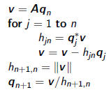
•Algorithm: Arnoldi Iteration
given random nonzero b, let
for n = 1 to 1, 2, 3,.....


Lanczos Iteration for Symmetric Matrices
•For symmetric A, and H_n are tridiagonal, denoted by and T_n,
respectively. AQ_n = Q_n+1 can be written as three- term recurrence

•where are diagonal entries and are sub-diagonal entries of
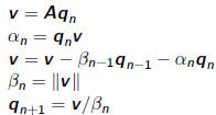
•Algorithm: Lanczos Iteration

given random b, let
for n = 1 to 1,2,3,....

Question: What are the meanings of and in ?

Properties of Arnoldi and Lanczos Iterations
•Eigenvalues of H_n (or T_n in Lanczos iterations) are called Ritz values.
•When m = n, Ritz values are eigenvalues .

•Even for n << m, Ritz values are often accurate approximations to
eigenvalues of A!

•For symmetric matrices with evenly spaced eigenvalues, Ritz values
tend to first convert to extreme eigenvalue.

•With rounding errors, Lanczos iteration can suffer from loss of
orthogonality and can in turn lead to spurious “ghost” eigenvalues.

Arnoldi and Polynomial Approximation
•For any

•It can be interpreted as a polynomial in A times b , x = p(A)b, where

•Krylov subspace iterations are often analyzed in terms of matrix
polynomials.
•Let Pⁿ be the set of polynomials of degree n with c_n = 1.
•Optimality of Arnoldi/Lanczos approximation: It finds s.t.
•p* is optimal polynomial among that minimizes ,
which is equivalent to minimizing the distance betwen Anb and its
projection in K_n
•p* is the characteristic polynomial of Hn
Ritz values are the roots of an optimal polynomial

2 Conjugate Gradient Method

Krylov Subspace Algorithms
•Create a sequence of Krylov subspaces for Ax = b

and find an approximate (hopefully optimal) solutions x _n in K_n
•Only matrix-vector products involved
•For SPD matrices, most famous algorithm is Conjugate Gradient (CG)
• method discovered by Hestenes/Stiefel in 1952
•Finds best solution in norm
•Only requires storing 4 vectors (instead of n vectors) due to three-term
recurrence

Motivation of Conjugate Gradients
•If A is m x m SPD, then quadratic function

has unique minimum
• Negative gradient of this function is residual vector

so minimum is obtained precisely when Ax = b
•Optimization methods have form

where p_n is search direction and is step length chosen to minimize

• Line search parameter can be determined analytically as

•In CG, p_n is chosen to be A-conjugate (or A-orthogonal) to previous
search directions, i.e., for j < n

Conjugate Gradient Method
 

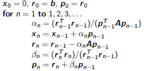
Algorithm: Conjugate Gradient Method
	step length approximate solution residual improvement this step search direction

•Only one matrix-vector product Ap _n-1 per iteration
•Apart from matrix-vector product, operation count per iteration is
O(m)
•If A is sparse with constant number of nonzeros per row, O(m)
operations per iteration.