1. MOTIVATION AND AN EXAMPLE
One of the most important objects in mathematics is the
univariate polynomial

Univariate polynomials occur in nearly all applications of
mathematics. The root of a polynomial
is the solution to the equation obtained by setting it equal to zero. It is easy
to solve
equations involving linear polynomials (mx + b = 0). It is almost as easy to
solve equations
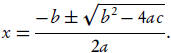
involving quadratic polynomials (ax2 + b x +c = 0) by the quadratic formula:
This is an example of solving an equation by radicals. It
is possible to solve cubic and quartic
polynomials by radicals as well, but the procedure is sufficiently complicated
that we now
consign this drudgery to a computer.
In the 19th century Niels Abel, Evariste Galois, and Paolo
Ruffini showed that a polynomial
of degree n > 4 cannot be solved by radicals. The solutions do exist, and we
need to work
with them! Since we cannot find the solution by radicals, our workaround is to
approximate the
solutions within a specified margin of error, .
Isaac Newton had already developed such a technique to
approximate real-valued solutions to
polynomials. Newton’s idea was to use the fact that the tangent line moves in
the same direction
as the curve to obtain a path towards the solution.
Example 1. Let
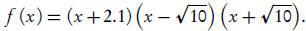 We see immediately that it has three
roots: x = −2.1, x =
 and x = −
Polynomials are not always expressed in this convenient
form, however. It is more common
to seem them expanded :
f (x) = x3 +2.1x2 −10x −21.
Factoring thiswould be very painful. Since it is a cubic,
one root must exist; plotting the function
shows that three roots exist. See Figure 1.
We will use Newton’s insight to approximate a positive
root. What is our goal? We would like a
value x = a > 0 such that f (a) ≈ 0. How close to 0 should we be before we think
we are close
enough? This depends on the application; for now; suppose we accept | f (a)| <
ε =
0.01. That
will keep the y-value within one-tenth of the desired value.
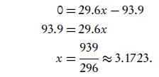
Start by plotting the tangent line at x = 3. Since
f ' (x) = 3x2 +4.2x −10,
we know that the slope of the tangent line is f ' (3) =
29.6. Since the y-value at x = 3 is
f (3) = −5.1, we have the equation
y +5.1 = 29.6 (x −3)
 y = 29.6x −93.9.
Plotting this line around x = 3, we see how it follows the
curve and intersects the axis near a
root. See Figure 2.
The root of the tangent line gives us an approximation to
the actual root of f . We can solve
the linear equation to find this approximation:
Is 3.1723 the actual root? We can decide by evaluating f
at 3.1723:
f (3.1723) ≈ 0.3347 ≠ 0.
So 3.1723 is only an approximation to the root. It isn’t a
satisfactory approximation, since we
want f (a) < ε= 0.01. If a = 3.1723 we have instead f (a) > 0.3 > ε!
Can we get do any better by repetition? Build another
tangent line, using the facts that
f (3.1723) ≈ 0.3347 and f ′ (3.1723) ≈ 33.5141.
This gives us the line
y −0.3347 = 33.5141 (x −3.1723)
y = 33.5141x −105.9821.
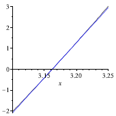
Glance at the graph again , in Figure 3. The line and the
curve are nearly indistinguishable!
Solving for the line’s root, we obtain the approximation
0 = 33.5141x −105.9821
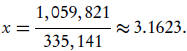
How close are we to a root? Substituting into f , we find
that
f (3.1623) = 0.0007.
This is a much better approximation; now | f (a)| < ε. We
are “close enough” to the real root, so
we stop.
2. OUTLINE OF THE METHOD
Newton’s Method is a simple, repetitive process. Given a
function f , we want an approximation
a to a root of f , with error no greater than ; that is, | f (a)| < ε. We
followed these
steps:
(1) Make a rough guess to an x-value that is root; call
this guess x = b.
(2) Calculate the y-value, f (b).
(3) If | f (b)| ≥ε, refine the approximation:
(a) Calculate the slope m of the tangent line at x = b.
(b) Using m and f (b), find the root of the tangent line. Call it b, and return
to step 3.
(4) Otherwise (| f (b)| <ε ), our answer is x = b.
We call this an iterative process because step 3 repeats .
The values x = b are called iterates. We
can label them as
• b0 for the initial guess;
• b1 for the first tangent line’s root;
• b2, for the second tangent line’s root; etc.
A large number of mathematical techniques are based on
iteration. Such techniques appear in
applications of mathematics. For example,
• in Graph Theory, we can use the Repetitive Nearest
Neighbor algorithm to solve the
Traveling Salesman Problem;
• in Modern Algebra , we can use the Euclidean algorithm to find the greatest
common
divisor of two elements in a Euclidean Domain;
• in Numerical Analysis , we can use the Conjugate Gradient Method to approximate
a
minimum value of a function.
3. IMPLEMENTING AN ITERATIVE PROCESS IN PSEUDOCODE
Pseudocode gives us the while keyword to indicate that a
process should repeat:
while condition
instruction 1
instruction 2
instruction 3
indicates that as long as condition remains true, we should repeat instructions
1 and 2. Once
condition becomes false, we proceed to instruction 3. For example,
a := 24
b := 15
while b ≠0
r := a mod b
a := b
b := r
return i
implements the Euclidean algorithm to find the greatest common divisor of 20 and
15.
Try to follow the pseudocode given above. Remember to repeat the instructions
inside the
while until b = 0. Make sure that you understand how we obtain the following
values of a, b,
and r :
NEWTON’S METHOD 4
| iteration |
a |
b |
r |
| 1 |
24 |
15 |
9 |
| 2 |
15 |
9 |
6 |
| 3 |
9 |
6 |
3 |
| 4 |
6 |
3 |
0 |
| 5 |
3 |
0 |
- |
4. EXERCISES
Exercise 1. Given a guess bi , find a formula for the next guess bi+1 in
Newton’s Method. Use
the fact that bi+1 is the root of the line tangent to f at x = bi .
Exercise 2. Write an algorithm for Newton’s Method using pseudocode.
Some remarks on this exercise:
(1) Be sure to identify the inputs and the sets. You need three.
(2) To tell the computer how to make its next guess, you can use either the
formula you
found for Exercise 1, or a translation of step 3 in Section 2.
(3) Although lines 3–4 are written with the words if/else, it would be incorrect
to use the
if/else pseudocode to implement them. Why not? Pseudocode doesn’t have step
numbers,
so you have no way of writing “return to step 3”. However, returning back to a
certain
step usually means repeating several steps as long as a certain condition is
true. Thus,
your pseudocode should use the keyword for repetition, not the keyword for
decisionmaking.
Exercise 3. Translate your pseudocode for Exercise 2 into a Maple program. Test
the program
on the inputs f and b given in Example 1, to make sure that you have the correct
output.
Exercise 4. Use your program to try to approximate a root for each of the
following functions,
with = 0.0001:
(a) f (x) = 2x −3.
(b) g (x) = x2 −2.
(c) h (x) =
x6+0.04x5−1.99962x4−0.0800008x3+1.001219992x2+0.0400008x+0.000400008.
Exercise 5. One sometimes has to be careful when trying to apply Newton’s
Method. Some
functions will not work at all; others will work only with special inputs.
(a) Explain why it is a very bad idea for the first guess b to satisfy the
condition f ′ (b) = 0.
(b) Find a bad first guess for Exercise 4(b).
(c) What happens in your program when you try Exercise 4(b) with this bad first
guess?
(d) Experiment by hand using Newton’s Method with
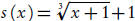 and first guess b = 0.
What happens in this case?
(e) What happens in your program when you try s with the first guess b = 0 and ε =
0.1?
Exercise 6. Amore common implementation ofNewton’s Method is to continue
approximating
until a certain number of digits do not change. In the example given, notice
that the four digits
beyond the decimal change with each iteration : 3.000, 3.1723, 3.1623. If our
goal is to have an
approximation a that is accurate up to four digits beyond the decimal point, we
may have to
proceed further.
(a) Write new pseudocode for Newton’s Method that checks for this new condition
rather
than for f (a) < ε. Notice that you have to change the inputs! Instead of
ε, a
margin of error,
you need d, a number of digits.
(b) Implement the pseudocode in Maple. You can use Maple’s round() function to
round to a
certain number of digits. Try it on each of the examples of Exercise 4, with 6
digits of accuracy
beyond the decimal point.
Exercise 7. Sometimes we want to identify a particular root, but it is hard to
find a starting
point. Consider
f (x) = x4 −0.0221x2 +0.000121.
This function has four real roots, all of them relatively close to zero . It is
not easy to approximate
the two roots closest to zero.
(a) Use your program from Exercise 6 to approximate all four real roots , with 8
digits of
accuracy beyond the decimal point.
(b) Plot the graph of f around the four roots. Try to explain, using calculus,
why it is hard to
approximate two of the roots.
FIGURE 1. Diagram of Newton’s Method: initial graph of f .
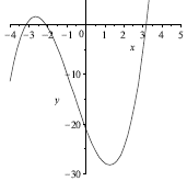
FIGURE 2. Use the line tangent to f at the first guess (x = 3) to obtain the
second
guess (x = 3.1723).
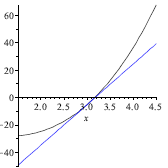
FIGURE 3. Use the line tangent to f at the second guess (x = 2.87) to obtain the
third guess (x = 3.19).