Mathematical Induction

Theme 1: Principle of Mathematical Induction

Mathematical induction is used to prove statements about natural numbers. As students may remember,
we can write such a statement as a predicate P(n) where the universe of discourse for n is the
set of natural numbers

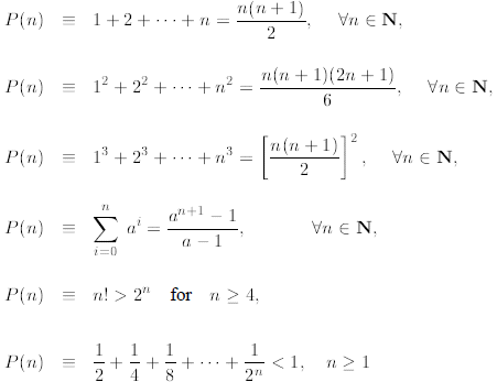
Example 1: Here are some examples of what we mean by P(n):

where means “logically equivalent”.

The first three expressions above provide closed-form formulas for the sum of n consecutive
positive integers, the sum of squares of n consecutive positive integers, and the sum of cubes of
n consecutive positive integers, respectively. The fourth expression is the sum of the first n terms
in the geometric series and we studied it already in Module 2. The last two expressions are useful
inequalities for factorial and the sum of negative powers of 2.

Every statement P(n) above is about natural numbers or a subset of natural numbers (e.g., for
n ≥4). How can we prove such statements? Consider the first example above regarding the sum of
the first n consecutive positive integers. We can easily verify that P(n) is true for some selected n.
Indeed,

P(1) is true since

P(2) is true since

P(3) is true since

But how can we prove that P(n) is true for all n ∈ N?

The principle of mathematical induction (PMI) can be used to prove statements about natural
numbers.

The principle of mathematical induction: Let A be a set of natural numbers such that
the following two properties hold:

(1) 1 ∈ A;

(2) for every natural number n

if n ∈ A then

Then

that is, A contains all natural numbers.

How is it related to proving statements like P(n) above? Let us define

A ={n : P(n) is true for },

that is, A is the set of natural numbers for which P is true. The goal is to show that A is the same as
the set of all natural numbers, that is, A = N. Imagine that one verifies that P(1) is true. Then we
can set . Let’s now assume that one can prove step (2) of PMI (that we shall call the inductive
step). Thus since we know that 1 ∈ A, and we know the inductive step is valid, say for n = 1, we
conclude that 2 ∈A. Therefore, , that is, P(1) and P(2) are true. But using again the
inductive step, we conclude that 3 ∈ A. Etc. Actually, PMI allows us to replace the imprecise “etc”
by A = N, that is, P(n) is true for all natural numbers!

But why is PMI true, in the first place? We demonstrate its truth using the proof by contradiction.
Suppose that (1) and (2) of PMI hold but A is not equal to N. Hence, it must be at least one natural
number is omitted from N. Let n₀ be the first number (smallest) among 1, 2,... omitted from N. We
know that n₀ cannot be 1 since we assumed that 1∈ A by (1) of PMI. But by our construction, n₀ -
1 ∈ A. Then by step (2) of PMI we must conclude that n₀ ∈ A, which is the desired contradiction.
Therefore, A = N.

Let us introduce some additional notation. The first step (1) of PMI is called the basis step, while
the second step is known as the inductive step. It is usually trivial to verify the basis step, and most
work has to be done to prove the inductive step. We shall illustrate it on the following example.

Example 2: Prove the first identity above about the sum of n consecutive natural numbers, that is,

In this case, the property P(n) is a predicate saying that the above is true for n, and

A = {n : identity above is true for n ∈ N}.

We prove P(n) is true for all n (i.e., A = N) using PMI. We need to go through the basis step and
the inductive step.

Basis Step: We must prove P(1) is true, but this was already established before.
Inductive Step: We now assume that P(n) is true for a fixed but arbitrary n. The above assumption
is called the inductive hypothesis and in our case it takes the following form

for arbitrary n. (In the above symbol := means equal by definition.) The reader must understand that
the statement immediately above and the statement that we want to prove are not the same, even if
they look alike. In the statement above we assume that the identity to be proved (about all sums of
the first n consecutive natural numbers) is true for one value of n (but an arbitrary one).

We now perform the inductive step. We must establish the inductive step, that is, to show that the
formula for S_n above implies that

is true, too. Observe that above we replaced n by n +1 (on the left-hand side of the equation as well
as on the right-hand side). Indeed, we have

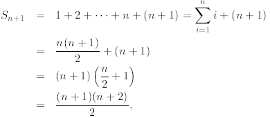
where in the second line above we invoked the induction hypothesis, in the third line we factored out
the term (n + 1), and then added what is left. This is exactly what we need to prove the inductive
step.

But, there is actually another, direct, proof originally proposed by the 18th century mathematician
Carl Friedrich Gauss. Let, as before, We write the sum S_n twice one starting the sum
from 1 up to n, and the second time starting from n down to 1. Then, we add the individual elements
vertically. Here is what comes out:

Since there are n terms (n + 1) in the bottom line, we prove that

Again, we recover the same identity.

Exercise 4A: Using mathematical induction prove that

Exercise 4B: Using mathematical induction prove that

Induction on a Subset of Natural Numbers

In the PMI discussed above in the first step we assumed that 1 ∈ A, however, if we start the induction
from another natural number, say k, then it holds for all n≥ k. This is shown in the next example.

Example 3: Prove that

for

We recall that We are asked to prove the above inequality only for
n≥ 4. Thus let

is true for

We first check that thus P(4) is true. (Observe that P(3) is not true.) Now
assume this statement is true for arbitrary n≥ 4. We must prove that

for n≥ 4. This is easy since

The first inequality follows from the induction hypothesis while the second identity is a
consequence of (n + 1) > 2 for n ≥4. This proves the desired inequality for all n≥ 4.

The next two examples require a little bit of work before the induction can be applied.

Example 4: Bernoulli’s inequality. We shall prove the following result.

Theorem 1 If n is a natural number and 1 +x > 0, then

Proof. The proof is by induction. In the basis step, we assume n = 1and verify that
is true for 1 +x > 0. Now, we assume (inductive hypothesis) that is true for an
arbitrary n, and we must prove that

for 1 +x > 0. To prove this we proceed as follows:

by induction

since 1 +x > 0

where the first inequality is a consequence of the induction assumption (i.e., we know that
1+nx so we can replace by 1+nx because 1+x > 0; observe that if 1+x < 0, then we
had to reverse the inequality sign). The next step is simple algebra, while the last step follows from
the fact that nx² is nonnegative; it doesn’t matter what the value of x, because for any
a. This proves the theorem.

Example 5: Let us prove that

for n ≥1. We prove it by induction. The first step for n = 1 is easy to check, so we concentrate on
the inductive step. We adopt the inductive hypothesis, which in this case is

and must prove that

A natural approach fails. If we invoke the induction hypothesis to the first n terms of the above, we
will get

which does not imply that it is less than or equal to 1 since Here’s how we proceed

by induction

<

≤1,

where in the first line on the right-hand side we factor 1/2 and observe that what is left in the parenthesis
must be smaller than 1 by the inductive hypothesis. The rest is simple algebra. This proves the
inequality.

In some cases, we must use a generalized mathematical induction that we formulate in a little
different form than before.

If a statement P(n) is true for n = 1, and if for every n > 1, the truth of P(n) for all
natural numbers < n implies the truth of P(n) for n, then P(n) is true for all natural
numbers.

The only difference between the basis PMI and the above is that in in the inductive step of the generalized
mathematical induction we assume that the truth of implies the
truth of P(n). In other words, the second step of the generalized PMI can be written as

then n ∈ A

where A is the set defined in the original PMI.

Recurrences

We now apply mathematical induction to establish some facts about recurrences. We come back to
recurrences in Theme 3.

We start with an example that illustrates an application of the generalized mathematical induction.

Example 6: Let us define T(0) = 1 and then

This is an example of a recurrence that we shall study in some details later in this module. Observe
that we can compute consecutive values T(1), T(2) and so on from the recurrence itself. For example,

But can we guess how T(n) grows for arbitrary n. In the table below we computed some numerical
values of T(n) and compared them to the growth of n and n².

n	T(n)	n2
1 3 6 9 12 15 18	3 7 13 19 25 31 37	1 9 36 81 144 225 324

From this table we should observe that T(n) grows faster than n and much slower than n². Let us
then conjecture that

We now use mathematical induction to prove this guess. Observe that
(since ), but , therefore, we must start the induction from n = 2.

To carry out the inductive step we shall assume that for all the above guess is is true.
We now prove that this guess is also true for n. Indeed,

induction

=

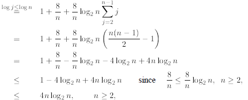
where (i) in the first step we use the recurrence and extract the first two terms from the sum; (ii) in the
second line we use the induction assumption in its general form and bound every T(j) by
for 2≤ j < n; (iii) in the third line we observe that(since j ≤n) and factor the
constant term in front of the sum; (iv) in the fourth line we apply the formula for the sum of
the first n - 1 consecutive integers proved in Example 2; (v) the fifth line is simple algebra; (vi) in
the sixth line we observe that

for n ≥2 and therefore cancel out the terms 8/n; finally the last inequality follows from the fact that
for n ≥2. (As we said at the beginning of this subsection, if this derivation is too
involved in the first reading, the student can move forward to the next section since it will not be used
in the forthcoming discussion.)

Theme 2: Newton’s Summation Formula

From high school we know that

But what about a formula for

for arbitrary n. We shall derive it here, and it is called Newton’s summation formula.

Before we handle the general case of , we must introduce some new notation. In particular,

binomial coefficients also known as Newton’s coefficients. We define for natural k and n ≥k

where we remind that By definition 0! = 1. In literature the Newton
coefficients C(n, k) are also denoted as

From the definition we immediately find

But we shall also need the following lemma.

Lemma 1 For natural k and n

Proof. We give a direct proof. Observe that

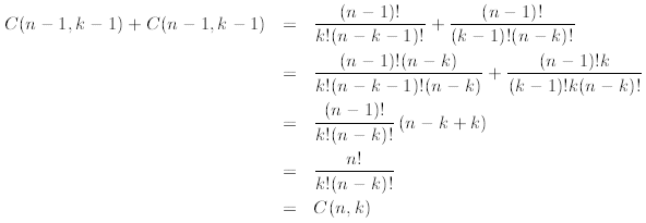
where in the second line we multiply and divide the first term by n - k and the second term by k.
Then we factorize and after some simple algebra obtain the desired result.

Now, we are ready to formulate and prove the Newton summation formula.

Theorem 2 For any natural n

Proof. The proof is by induction with respect to n. The basis step for n = 1 is easy to check since

C(1, 0) = C(1, 1) = 1.

We now start the inductive step, and postulate that if (7) is true for arbitrary n, then

must be true. We proceed as follows

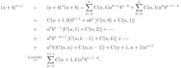
In the first line above we use mathematical induction and then multiply out. In the next few lines
we group terms with the same power, that is for all i. Finally, we applied Lemma 1 (i,e.,
C(n,k) + C(n, k - 1) = C(n+ 1, k)) to finish the derivation.

Exercise 4C: Apply Newton’s formula to the following

The above formula can lead to surprisingly interesting identities. Here are two of them

The first identity follows immediately from the Newton formula applied to

while the second follows from

We shall re-derive these identities using combinatorial arguments in one of the next modules.

Theme 3: Recursion and Recurrences

Sometimes it is difficult to define an object explicitly. In such cases, it is better to define this object
in terms of itself but of a smaller size. (Actually, we have seen this principle at work in mathematical
induction.) This process is called recursion and often it is described mathematically by a recurrence.

Example 7: Define a₀ = 1 and for n ≥0

Let’s see what we get. We first compute some sample values:

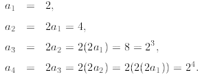
Based on this numerical evidence, we conjecture thatWe can prove it using mathematical
induction. But, in this it is easier to give a direct proof that is called telescoping. We proceed as
follows:

In the above we successively used the recurrence until we reached the initial value a₀ and
we know that a₀ = 1. Observe that without knowing a₀ we can neither start the recurrence nor finish
it.

Exercise 4D: Derive an explicit formula for the following recurrence for n ≥1

with a₀ = 1.

We can define some other functions recursively. For example, F(n) = n! can be defined recursively
as follows

Furthermore, let

where  is a given sequence. For a computer to understand such a sum, we must define it
recursively. For example, we can do it this way

But, let us consider a more general recurrences. We underline that in order to start a recurrence we
must define some initial values, and to provide a “method” how to compute the next value. Consider
the following recurrence

This recurrence starts with

1, 3, 7, 15,...

but what is a general formula for a_n? Let us move the term to the other side of the recurrence
and write down all the values as follows

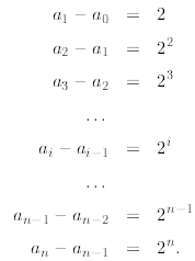
Now, when we add all these equations together most of them will cancel out (we say that the sum
telescopes) except a_n and a₀ giving us

which is the same as saying

Is this better than the original recurrence? Not yet since we must compute the sum. Actually, in
Module 2 we defined the geometric progression as follows

and we derived

Actually, we shall re-prove this formula using mathematical induction. It is easy to check its truth for
n = 0 (the basis step). Let us move to the inductive step. We first assume that the statement above is
true for arbitrary n, and we try to prove that this would imply that

We proceed as follows

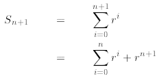
induction

=

where in the second line we extract the last term from the sum and write it separately as, then
in the next line we apply to the first sum the inductive hypothesis, and finally after some algebra we
prove the desired formula.

Now, we can return to (10) to conclude that

Let us solve some more recurrences. This is the only way to learn how to handle them. Let b₀ = 0
and

We do the following telescoping
 

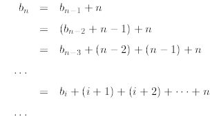
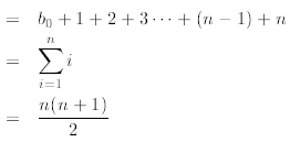
where in the second line we substitute in the third line we start observing
a pattern in which b_i is followed by the sum of the first i + 1 natural numbers. Then we apply the
sum of n consecutive natural numbers derived in Example 2. In every step of the above derivation we
used the recurrence itself to reduce it until we reach the value that we know, that is, b₀. We can do it
since in step i we know that

Consider now a more complicated recurrence:

Let us start the telescoping process and try to find a general pattern. We have

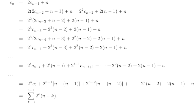
In the second line above, we substitute by and observe that the “additive term”
is now n+2(n - 1) (the additive term is the one that does not involve c_i). After another substitution
the additive term is enlarged to Now you should be able to see the pattern
which becomes After the last substitution
the additive term is finally

Now to finish the recurrence we must find a formula for the following sum

Observe that in the first sum we could factorize n since the summation is over k, thus n is fixed. After
this observation, the first sum is easy to estimate. We just found above that it is equal to . But
the second one is harder. To estimate it we first observe that

Then

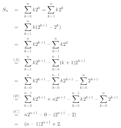
In line (A) we change the index of summation from k to k + 1, in line (B) we expand the first sum
and observe that it cancels out the second sum, finally in line (C) we apply the geometric sum that we
already discussed above.

Coming back to the recurrence, putting everything together we have

which is our final answer. Uffff ... it was not that hard.
Finally, we solve one non-linear recurrence. Consider the following6

where a₀ = 1. It is a non-linear recurrence since is squared. Telescoping might be difficult for
this recurrence. So we first simplify it. Define Then we have

sinceNow we are on familiar grounds. Using telescoping we find

which implies

Finally, we should say it is always a good idea to verify numerically our solution by comparing its
some initial values to the values computed from the recurrence itself.